Building a model to predict EC in hydroponic nutrient solutions
Electrical conductivity (EC) is one of the most useful parameters in the practical preparation of hydroponic nutrient solutions. This is because knowing the expected conductivity of a nutrient solution can allow you to prepare solutions without having to measure the total volume exactly, a parameter that is often hard to accurately determine in practice. Although determining the target conductivity is easy to do using small preparation volumes – which can be done accurately – it is often impractical to do so routinely, which is necessary if the actual composition of the nutrient solution is being changed as a function of time. Due to all the above, it is important to come up with accurate models to estimate the EC of nutrient solutions with only information about their mineral composition, without having to measure the value experimentally. In this post I am going to talk about how I created a model to do exactly this, taking advantage of multi-variable experimentation and simple modeling techniques.
The problem with conductivity modeling is that not all salts contribute the same to the conductivity of a nutrient solution. For example potassium sulfate can contribute significantly more to conductivity per gram compared to a salt like monopotassium phosphate. Furthermore, the addition of some salts can affect the conductivity of others (see my previous post on conductivity modeling in Hydrobuddy for more details). In the regime we use in hydroponics, the determination of electrical conductivity using data from limiting molar conductivity can lead to very skewed results, which makes these estimations of little usage in practice.
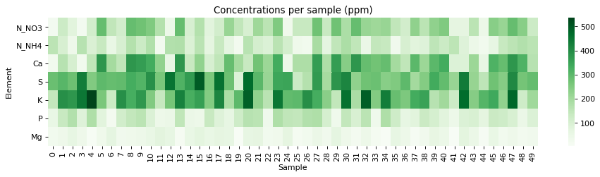
To solve this issue, I designed an experiment where 50 different EC measurements were made for different hydroponic nutrient solutions within the range of concentrations of nutrients that are reasonably expected in hydroponic culture, with some values being above these in order to ensure that all values encountered in practice will be within the measured ranges. The image above shows you all the concentrations that were measured within the experiment. To prepare the solutions I used calcium ammonium nitrate, potassium sulfate, magnesium sulfate heptahydrate, monopotassium phosphate and ammonium sulfate. All of these were agricultural grade salts in order to reflect the same impurities expected in a normal hydroponic setup. Note that no heavy metal salts were used since their contribution to the EC of a hydroponic nutrient solution is negligible.
Concentrated solutions of all the salts were prepared in 250mL volumetric flasks using a +/-0.001g scale and aliquots of these solutions were drawn using 5mL plastic syringes (+/- 5%) in order to prepare final 250mL solutions using volumetric flasks. Conductivity measurements were done using an Apera EC60 conductivity meter that was previously calibrated using a 2 point calibration method. All the solutions were prepared using distilled water. The target concentrations for the solutions were determined using a pseudo random number generator in order to try to ensure a random distribution of samples within the concentration space of interest.
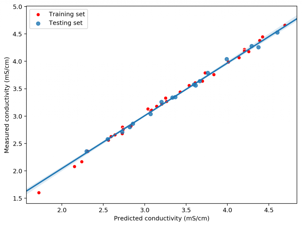
Using this data we constructed a linear model to attempt to predict conductivity. In order to evaluate the model we randomly split the results to get 33 data points used for model construction and 17 points left for model validation. Performing this process 100 times shows that the mean R2 of the model on the training set is 0.995 while the average on the training set is 0.994. This shows that the model is able to properly generalize the conductivity data in order to properly predict the conductivity of the solution across the space studied. The mean absolute error in the testing set was 0.036 mS/cm. This shows the high certainty with which we can make conductivity predictions.
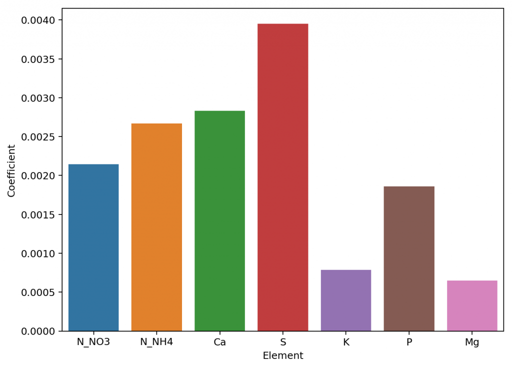
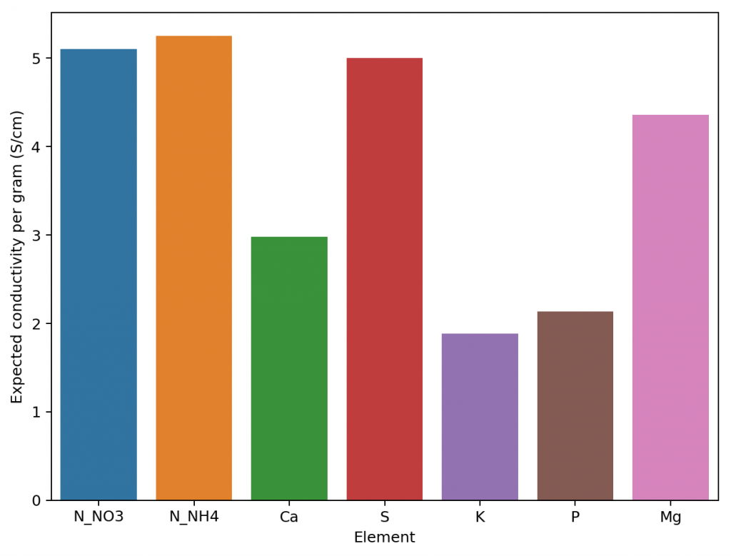
Exploring the model coefficients can also show us how different the contributions of the different elements to the conductivity of the nutrient solution can actually be. These results are surprising if you compare them to the conductivity contributions per gram that are expected from the limiting molar conductivity values, which are the conductivity values the ions exhibit on their own under very high dilutions (this is also the method used in HydroBuddy <=v1.65). We can clearly see here that in reality we are getting way more conductivity out of sulfate compared to the other elements and significantly less from magnesium. This means that at the makeup and concentration values used in hydroponics the Mg ions are not being able to contribute as much as they can when they are alone because their activity is being lowered by the other ions in solution, while the opposite case applies to sulfate.
The above shows us why conductivity in hydroponics is so complicated, it shows how ions do not contribute equally to conductivity and how they behave very differently in real hydroponic solutions. Thankfully the above also shows how we can create a model using experimental data that is actually able to predict conductivity, since the relationships – although different than expected – are still highly predictable when enough experimental data is available. All the above experimentation took 4 hours to do – with the help of my lovely wife, who is also a chemist – and should allow me to add a very powerful model to predict hydroponic nutrient solution EC values to HydroBuddy.
All the above experimentation data will be open source and available in a github repository soon. We also hope to show you how all of this was done in a youtube video in the near future.