Problems are an inevitable part of being a hydroponics grower. Even experienced growers will sometimes face issues when moving between environments or plant species as things change and new challenges arise. A big part of being a good grower is to be able to think about these obstacles, find out their causes and successfully respond to them. In this post I want to share with you some information about the data you should gather in order to properly diagnose a problem in your hydroponic crop. This is important as not having enough data often makes it impossible to figure out what’s going on, while simple measurements can often give a very clear view of what’s happening with the plants.

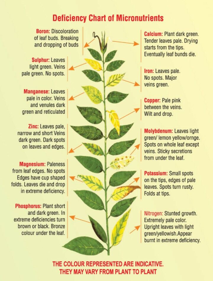
Take detailed, well documented pictures. What you see is a very important portion of what describes a plant’s status and issues. The first thing you should do is document what you’re seeing – take pictures of the plants showing the problem – and write down the symptoms you are observing. This documentation process should be organized, give each plant an ID, take pictures under natural light or white light of the new leaves, old leaves and root zones (if possible). Take pictures across different days showing the evolution of symptoms. Have all this information so that you can then better interpret what is going on. Also remember that symptoms do not necessarily mean deficiencies and deficiency symptoms does not necessarily mean more of a nutrient needs to be added to a nutrient solution (for example a P deficiency can show under low nutrient solution temperature even if P in the solution is actually very high).

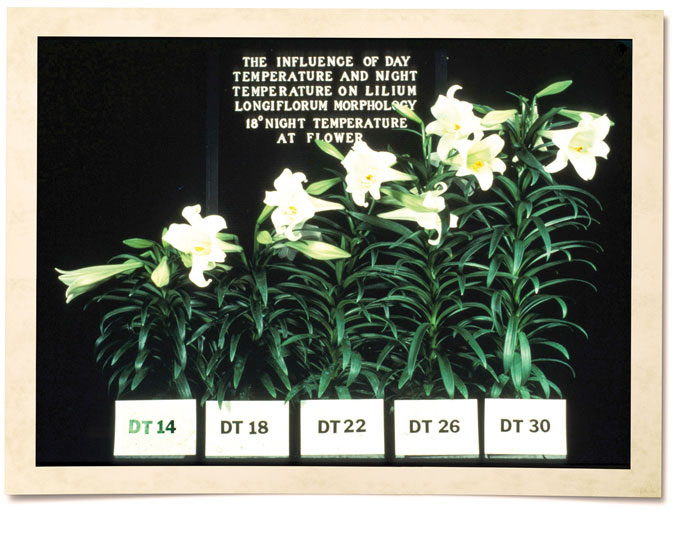
Record all environmental data. When a problem happens, it is often related to the environment the plants are in. Having recorded data about the environment is a very important part of evaluating the issue and figuring out what went wrong here. Getting a good view about the environment usually involves having measurements for room temperature, temperature at canopy, relative humidity, carbon dioxide concentration, nutrient solution temperature, PPFD at canopy, and root zone temperature. All of this data should be recorded several times per day as they are bound to change substantially between the light and dark periods.

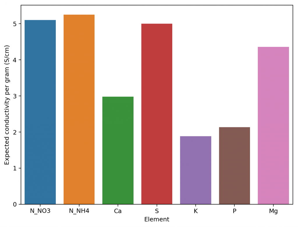
Get nutrient solution analysis. Diagnosing a problem is all about having a complete view of what’s going on with the plants. The nutrient solution chemistry can often be a problem, even without the grower knowing a problem is brewing there. Sometimes nutrient solution manufacturers might have batches with larger errors than usual, or the input water might have been contaminated with something. There is also the potential of human error in the preparation of the solutions, which means that getting an actual check of the chemistry of the solution can be invaluable in determining what’s going on.

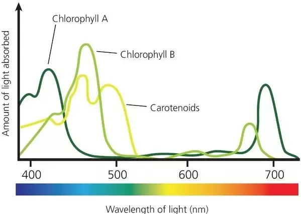
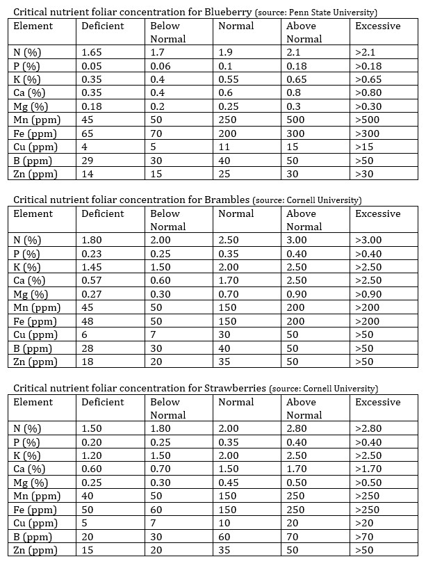
Get leaf tissue analysis. Even if the nutrient solution analysis does not reveal any problems, there are often issues with plants that are related with interactions between the environment and the solution that can go unnoticed in a chemical analysis of the solution itself. Doing a leaf tissue analysis will show whether there are any important nutrient uptake issues within the plant, which will provide a lot of information about where the problem actually is.

Take well documented pictures of tissue samples using a microscope. A microscope can be important in determining what’s going on with plants, because it can show developments in roots/tissue that cannot be seen with the naked eye. Microscopes can often reveal very small insects or fungal structures that would have otherwise gone unnoticed. For this reason, a microscope and the taking of microscopy images can be of high value when dealing with a problem in a hydroponic crop.

With all the data mentioned above, most hydroponic crop problems will be much easier to diagnose. Some of the biggest failures in dealing with problems in hydroponic crops come from not gathering enough data and just guessing what the problem might be given how the plants look. Sadly plants can show similar responses to a wide variety of problems and – in the end – nothing replaces having the data to actually diagnose what’s going on in order to deal with the issue appropriately. Lacking an evidence-based picture is often the biggest difference between success in diagnosing/fixing an issue and failure or even worse problems caused by taking actions that have nothing to do with the real problem at hand.

Controlling an entire hydroponic crop using electronics is not a trivial task. This includes everything from the automated control of things like relative humidity and ambient temperature, to other variables, such as lights, solution pH, conductivity and temperature. Many paid solutions exist in the market, but, in my experience, none of them offer enough flexibility to accommodate all potential environments, as all the ones I know are closed source and do not allow users to readily modify the firmware/software used to fit the user’s particular needs. Through the past 5 years I have setup control infrastructures across several different crops and have usually done so using an entirely DIY infrastructure that focuses on flexibility and power for the end user. In this post I want to talk about how this setup usually works and why I came to these design choices.

In general the infrastructure I setup relies on the use of wifi for the communication of the devices. This is because it’s usually the easiest to setup, although it might not be the most power efficient or the most desirable in all cases. I generally divide devices into three camps. There is a main device – which is usually a capable computer – which serves as the “central hub” for the entire setup. This computer contains the main database that stores all information about devices, sensor readings, calibration variables, alarms, etc and is in charge of deciding which control actions to take given the sensor reading it is receiving and the control devices it has access to. This central computer usually hosts a website as well, where the user can easily modify things, issue manual control actions, add new devices, set up alarms, etc. The computer can be duplicated as well, to prevent this from being an important point of failure. In several cases we have used a raspberry pi to play this role.

The second and third group of devices are usually Arduinos whose main role is to either take readings (measuring stations) or execute control actions (control stations). Some arduinos might actually serve both purposes as an arduino can often be fit with things like pH/EC probe readings as well as relays that control peristaltic pumps that are used to push pH up/down or nutrient solution into a solution tank. It is worth noting that the decision of what to do for control is never taken by any control station but all they do is interpret control messages from the computer and then try to execute those actions and then give back some response of what’s going on. Measuring stations, on the other hand, are only trusted with the task of taking some measurement from the environment and broadcasting it to the network, the only thing they might listen for are messages issued by the computer to modify their calibration, whenever this is required.

Measuring stations can be fully customized to have as many reading as the user desires and can be implemented to do all sorts of things, from measuring temperature and humidity, to measuring air-flow, to measuring media water content. This allows for dozens of different temperature and humidity reading spots using different kinds of sensors, to monitoring things such as irrigation flow and solution ORP and dissolved oxygen values.

The entire setup relies on the use of the mosquitto (mqtt) protocol in order to have each device brodcast a specific topic with a specific reading that other devices can subscribe to. The computer will listen to all the devices it sees within its database and it is therefore easy for a new device to be added by a user, since it only requires the inclusion of the device into the database. The measure/control stations can subscribe to the specific topics their interested in for calibration or control actions and can act whenever they receive these messages. All the devices are automatically added to a web platform and alarms can easily be set for any of the measurements carried out by the measuring stations.

A big advantage of this approach is that control actions can be made as complex as the user desires. This includes doing things like implementing reinforcement learning based controls for things like temperature/humidity allowing the computer to use a wide array of measurements in order to take control actions, not relying solely on the measurement of one limited sensor to make these decisions. This allows a computer to use information such as outside temperature to decide how much air it wants to get into the facility for control, or how long it wants to turn on humidifiers in order to allow the desired level of humidity within a grow room.

With all this said, DIY control is definitely not the easiest route to take. Implementing something like the above will require the purchasing of a lot of different electronics – which are sometimes expensive depending on what the user wants – and does require a lot of time programming firmware and deploying software so that the desired outcome can be achieved. With that said, the unparalleled level of control is often worth it and can be accompanied by substantial gains in the information available to the user, which often leads to improvements in yields and the significantly quicker catching of potentially important problems.

On the next part of this post, I will talk about some of the practical aspects of this project, such as which arduinos and sensors I usually use and how these are setup to communicate with the central computer. If you want to learn more about how I can help you set this up for your crop please feel free to contact me using the website’s contact form.

After many years of experience as a consultant in the hydroponic industry and interacting with dozens of different customers growing different plants with different systems, there are some common misconceptions that become apparent as time goes by. As a chemist, the ones I remember the most are related with the management of nutrient solution and the diagnosis and treatment of nutritional problems in plants. In today’s post, I want to talk about some of these misconceptions and hopefully shine light into what the more accurate interpretation of these phenomena actually is.

The EC is increasing, my plants are not feeding! One of the concerns I most commonly address is that plants are “not feeding” because the electrical conductivity (EC) of the nutrient solution is not decreasing, but actually increasing after the solution goes through the plants. Many growers think that EC measures nutrients in a solution, so if a plant feeds on nutrients, then the EC should naturally decrease as the plant feeds. This is wrong because the plant consumes both nutrients and water and EC is a proxy for nutrient concentration and not for the absolute amount of nutrients in the water. As a plant feeds it will absorb both nutrients and water but significantly more water than nutrients. Remember, plants are mostly made out of water and also use water to regulate temperature, humidity and nutrient uptake, so they will take way more water than nutrients, increasing the EC as they feed. As a plant grows larger it’s nutrient and water demands grow, but the water demand grows significantly more than the mineral nutrient requirements, meaning the plant will progressively increase the EC more and more as it feeds more and more aggressively.

The plants are yellowing, there must be a nutrient deficiency. As soon as plants start to show signs of yellowing, a significant amount of growers will immediately look and try to interpret this as a sign that there is some form of nutritional deficiency. Most that subscribe to this belief will look for pictures of deficiencies online and do their best to match what they see with a deficiency and then proceed to supplement the solution with some fertilizer that contains the “missing element”. More often than not, this is actually not caused by the composition of the solution at all but by some environmental factor that is not being properly managed. In run-to-waste systems this is most commonly related with a significant pH drift in the media – reason why it is always necessary to measure pH/EC of the run-off – but it can also be related to unnecessarily harsh VPD conditions or even a lack of enough air circulation. I would say that 5/10 times, problems with the plants have virtually nothing to do with the nutrient solution at hand.

If you want more X, then increase X in the nutrient solution. The relationships between the concentration of elements in a solution and the concentration of nutrients in plant tissue is not linear. Sometimes, increasing the concentration of an element in solution can actually lead to less of that nutrient being present within plant tissue. An example of this can be phosphorous, a plant can suffer from a phosphorous deficiency due to the formation of insoluble iron phosphate compounds in tissue that appear when the concentration of these two elements goes above some threshold. As more of either is added, more of these insoluble compounds are formed and less of P and Fe actually gets to the plant. Another example can be Ca, where the amount of Ca in tissue is more dependent on VPD than on the concentration of Ca in solution, changing the VPD by 20% will affect Ca in tissue significantly more than adding 20% more Ca to the solution in some plant species. In these cases you might add 20% more Ca but your VPD drops 20% and you actually see a decrease of Ca in tissue. Sadly nutrient dynamics are not simple and often a more holistic picture needs to be used to approach nutritional management!

Plants need aggressively more phosphorous when they flower. Most commonly used fertilizers in soil tend to have higher P/K values when they target “flowers”, this is because, in soil, phosphorous is not highly available and the supplementation of highly available phosphorous during flower can be very useful to plants. However, flowering plants in hydroponics always have access to significant amounts of soluble P and most actually do not require an increase from this base level when they go into their flowering periods. Many commercial hydroponic solutions used for tomatoes will – for example – keep their P values at 50 ppm through the entire growing period, only increasing K during the flowering period, but not P. Experiments across various commercially grown flowering species have shown that levels in the 50-65ppm range are ideal for many plants during their entire life cycle, this matches the experience of growers in the horticultural hydroponic industry.

There is a perfect nutrient solution. Many growers go on a “holy grail” quest to find the “perfect” nutrient solution that will give them the absolutely best yields. Many commercial fertilizer producers also call me asking to formulate “the best possible formulation” to grow a given type of plant or – even worse – to grow a wide variety of plants. The truth is that the ideal solution to feed a plant will depend on the genetics, the environment, the irrigation system, the growing media, etc. Due to the large amount of variability between growing setups, plant genetics and growing methodologies, more often than not, the nutrient optimization process needs to be carried out for every grower. Don’t get me wrong, a base formulation will probably get you 80% of the way to your maximum potential yields – nutrient solutions are not miracle generators, they are just food – but conquering that final 20% will require a lot of additional effort that will most likely be limited to your particular conditions. This is because most environments are limited by different factors and using the nutrient solution to help overcome some of these limitations will modify the solution in a way that’s probably detrimental for other environments.

I hope the above misconceptions show that the world of nutrient solutions and plant management is not so simple and that there is a lot that goes into understanding how nutrients interact within a plant and how a given growing environment needs to be modified in order to improve crop results. My goal is to help you expand your knowledge about hydroponics and better reach your goals by overcoming some of these misconceptions and tackling some of the true problems within your hydroponic crops.

Although a significant portion of hydroponic growers use run-to-waste setups – where the nutrient solution is ran through plants and then lost – the industry is now moving towards the implementation of recirculating hydroponic systems in order to reduce both water usage and the unnecessary dumping of fertilizers into sewage systems. A recirculating setup has many advantages and can provide better yields than run-to-waste setups, provided the solution is properly managed and changed through the growing cycle. In this post I’m going to talk about five tips that will help you successfully manage your nutrient solution when using this type of system.

Ensure the volume of the reservoir is at least 10x the volume necessary for a single irrigation. The total volume of a reservoir is key in a recirculating setup because you want the bulk of the solution to be unaffected by whatever nutritional changes are caused by the plants during each feeding. This means that you want most of the solution to be inside your tanks and not inside the media when every irrigation is done. A simple rule of thumb is to make the volume of your initial reservoir at least 10x the volume that it would take to carry out a single irrigation of your entire crop. If you do this the water and nutrient absorption effects will happen slowly and will give you time to manage your solution without any harm coming to the plants.

Circulate your solution until your pH and EC are constant. After an irrigation cycle starts, the solution will first mix with the remnants of the last irrigation cycle within the media, which will make the pH and EC of the return different from those of the main tank. In order to ensure that the plant’s root system is being subjected to the desired nutrient concentrations, make sure you carry out the recirculating process until the EC and pH of the tank remains constant and matches the return pH and EC. Once this happens you know that the conditions within the media have now been equalized with the larger body of solution and you can stop the irrigation process. Constant monitoring of the pH and EC within the tank are therefore necessary within this type of setup.

Add water and not nutrients when the EC increases with every irrigation. In a normal recirculating setup the EC of the solution in the main tank will tend to increase with every irrigation while the total volume of the solution will decrease. This happens because healthy plants always absorb more water than nutrients, which means any measure that’s proportional to concentration – such as the EC – will tend to increase as the amount of water goes down. You want to add enough water to bring the EC down to the desired EC but you do not want to add nutrients with this water and this would increase the EC or contribute to nutrient imbalances within the solution. Note that you will need to add less water than the amount that was absorbed by the plants, because the plants also take some nutrients with them, meaning that the amount of water needed to reestablish the EC to what it was before will be lower. If an initial solution has 1000 gallons, the volume might go down to 950 gallons on the first irrigation but you might only need to add 20 gallons to bring it back to the original EC, making the total in the end around 970 gallons. Make sure the pH of the tank is also corrected after every irrigation and water addition.

Replenish water with nutrients when volume is down 40%, use this as an opportunity to shift the solution. As discussed in the last tip, the volume of solution will go down with time, even if some water is added to return to the original EC. At some point more than 40% of the volume will have been spent and it is at this point where you should fill the tank back to its full volume with water plus nutrients. You can also use this opportunity to change the nutrient ratios and skew them in the direction that you want your plants to follow nutritionally. For example in a flowering crop it is common to increase the amount of potassium during the blooming stages of the plant, so this can be done as nutrient solution is replenished after it’s consumed by the plants. Note that this process cannot be carried out indefinitely because both nutrient imbalances and plant exudates will accumulate within the main solution. Most recirculating crops will fully change the solution every 3-4 weeks to avoid these problems although the life of the solution can be extended further when chemical analysis is done – to customize nutrient replenishing – and adequate filtering is implemented to remove substances contributed by plants.

Add in-line UV filters and carbon filters. It is fundamental to ensure no microorganisms contaminate your nutrient solution. For this reason, online UV-filters are necessary to keep the nutrient solution as sterile as possible. Carbon filters are also very useful as they remove plant exudates that can contaminate the solution and cause problems within the crop itself. Many of these exudates are food for microorganisms, others are plant hormones that might cause unwanted responses in the plants. However both carbon filtration and UV filters can cause some issues – such as the destruction and adsorption of heavy metal chelates – so it is important to use chelates that are more resistant to UV and have less affinity for carbon filters to alleviate these problems.

There is certainly a lot more to the management of recirculating hydroponic solution than what I have detailed above, it is important to note that some of these tips are simplifications and much better tailor-made solutions are possible with a proper analysis of each situation. These are just some simple tips to hopefully make your change towards the use of recirculating systems a lot easier and should greatly increase your chances of success in the world of recirculating hydroponic setups.

Hydrobuddy is an open source calculator that seeks to help growers create their own hydroponic nutrient solutions. In order to do this, the program includes a database with a list of curated fertilizers that should be a good starting point for those interested in making their own nutrients. However, why these salts are included might not be clear to most growers, so I wanted to create a blog post to explain my reasoning behind this particular repository and the purpose each one of these different salts might serve. It is also worth noting that the default list of nutrients is not by any means definitive – for example no silicon containing substances are included – so users are welcome to add their own substances using the “Add Custom” option and entering the composition of the fertilizer they want to add.

The idea of the database that comes with HydroBuddy is to allow you to create several types of nutritional tools, using different types of approaches. The table below shows you what each one of the substances contributes in terms of nutrition, as well as its qualitative effect on the pH of the solution and what its most popular use is. While some of these substances – such as Potassium Sulfate – are mainly intended to be used as part of the main nutrient solution, others such as Potassium Carbonate, are not intended to be used in this manner but they are intended to be used as buffering agents when doing pH adjustments or creating concentrated pH up/down buffering solutions. There are also substances like – like Ammonium Chloride – that are not intended to be used for either of these purposes but mainly for supplementing a nutritional component, in this particular case, N as ammonium.

The main nutritional use of substances is also dependent on what the end-user has in mind. For example when a user wants to create a concentrated stock solution, substances such as Calcium Sulfate or Zinc Sulfate might not be very useful – due to their limited solubility or stability – while for users who want to create final solutions by direct addition of salts, these substances might be the best potential choice. Several different substances are provided for some nutrients to allow for this type of flexibility.

Another important factor can be cost, sometimes this is a more important factor than other considerations, such as which nutrient is the absolute best from a botanical perspective. This is part of the reason why – for example – 4 different forms of iron are present within the default database, this way users can see how much iron they would require from different sources and – depending on their particular application and cost range – make a decision about which iron source might be optimal. This also allows a user to consider using a cheaper source of iron – like Iron II Sulfate Heptahydrate – and then preparing their own chelates using a chelating agent, such as disodium EDTA.

For those with experience in hydroponic nutrient solutions it will be clear that many commonly used substances are missing – such as Magnesium Nitrate, Potassium Silicate, Nitric acid, Sulfuric acid, etc – these were present in previous versions of the software, but the abundance of choices was confusing to newer users, especially when they couldn’t easily get their hands on many of these fertilizers from a practical perspective. Some nutrients, like urea, were specifically removed because of the larger potential to cause more harm than good when used in hydroponics.The modifications to the database seek to solve these issues by providing a more condensed, yet very flexible list, that users can more effectively leverage to create their own solutions. However, remember that you can add any substance you want by using the “Add Custom” button in the substance selection screen.

As you can see many considerations go into creating nutrient solutions and this database is a very generic attempt to provide you with the best tools to get you started in this world. However, if you find this task difficult or you would simply like to have additional help and guidance, feel free to book an hour of consultation time by using the booking function on the website or contacting me directly through the contact page.

On my previous post you can read about how I ran experiments to develop a conductivity model using empirical data in order to improve our ability to predict EC values from the concentration of individual nutrients in a hydroponic nutrient solution. In this post I will now talk about how this was finally implemented in HydroBuddy, what form it took and what kind of result can be expected from it. The implementation discussed in this post has already been updated to the HydroBuddy github along with all the experimental data used to derive this empirical EC model.

Given the amount of data and the nature of the problem at hand, the easiest and most accurate way to build a model was to use a simple linear regression algorithm. As previously shown this model was able to give great results within the data, even when performing random training and testing splits. I have added a jupyter notebook to the github repository, along with all the data we measured in order to allow you to see how all the calculations were done, how the model was created and the sort of accuracy the model got within the set of experimental results. You can also play with this notebook to develop your own models or analyse the data any further if you wish. You can also try to reproduce our experiments and help verify our results. The linear model was translated into FreePascal and added to HydroBuddy although the program still retains the ability to estimate conductivity using the previously available LMC based model.

The fact that we were able to create a model to accurately determine conductivity within this experimental space does not mean that this model will work to magically determine the conductivity of any hydroponic formulation. These experiments were designed using five salts – calcium ammonium nitrate, ammonium sulfate, potassium sulfate, magnesium sulfate and monopotassium phosphate – which means that although our model is able to greatly describe conductivity in this space, the model is likely to run into trouble when attempting to describe a space that deviates too strongly from the one described above. This will be most evident whenever there are some cations or anions that are not present at all within these experiments. For example when silicates, chlorides or other such salts are used or when strong acids or bases are added to the solution.

Another important issue is the way these ions are paired. In our experimental process the concentration of Ca and N as nitrate always increased at the same time, meaning that the linear model implicitly carries this assumption. A setup were magnesium nitrate or potassium nitrate are used as well, will contain deviations from the current model that it is likely not very well prepared to deal with. A similar problem might happen when salts such as ammonium monobasic phosphate are used, since our model only contained a single example of a phosphate salt (monopotassium phosphate). While it is not easy to predict how much accuracy will be lost in these cases, we do expect the model to be significantly more inaccurate as other salts are used.

Additionally, our experimental setup did not contain any corrections of pH values, so the conductivity values described include a pH drift related with the amount of acid contributed by the potassium monobasic phosphate, which was not neutralized by a base. This will also cause differences with conductivity, if the conductivity is measured after the pH of the solution is corrected to the proper range used within the hydroponic process. Although at the concentration values used in hydroponics this should not be a big issue, it is still something worth considering.

As I mentioned above, the model is already implemented within the github repository – if you want to compile the program yourself – but the binaries won’t be updated to v1.8 until later this week. I look forward to your feedback about the model and hope it can help – at least some of you – to dramatically improve the estimations of conductivity of your hydroponic nutrient solutions.

Electrical conductivity (EC) is one of the most useful parameters in the practical preparation of hydroponic nutrient solutions. This is because knowing the expected conductivity of a nutrient solution can allow you to prepare solutions without having to measure the total volume exactly, a parameter that is often hard to accurately determine in practice. Although determining the target conductivity is easy to do using small preparation volumes – which can be done accurately – it is often impractical to do so routinely, which is necessary if the actual composition of the nutrient solution is being changed as a function of time. Due to all the above, it is important to come up with accurate models to estimate the EC of nutrient solutions with only information about their mineral composition, without having to measure the value experimentally. In this post I am going to talk about how I created a model to do exactly this, taking advantage of multi-variable experimentation and simple modeling techniques.

The problem with conductivity modeling is that not all salts contribute the same to the conductivity of a nutrient solution. For example potassium sulfate can contribute significantly more to conductivity per gram compared to a salt like monopotassium phosphate. Furthermore, the addition of some salts can affect the conductivity of others (see my previous post on conductivity modeling in Hydrobuddy for more details). In the regime we use in hydroponics, the determination of electrical conductivity using data from limiting molar conductivity can lead to very skewed results, which makes these estimations of little usage in practice.

To solve this issue, I designed an experiment where 50 different EC measurements were made for different hydroponic nutrient solutions within the range of concentrations of nutrients that are reasonably expected in hydroponic culture, with some values being above these in order to ensure that all values encountered in practice will be within the measured ranges. The image above shows you all the concentrations that were measured within the experiment. To prepare the solutions I used calcium ammonium nitrate, potassium sulfate, magnesium sulfate heptahydrate, monopotassium phosphate and ammonium sulfate. All of these were agricultural grade salts in order to reflect the same impurities expected in a normal hydroponic setup. Note that no heavy metal salts were used since their contribution to the EC of a hydroponic nutrient solution is negligible.

Concentrated solutions of all the salts were prepared in 250mL volumetric flasks using a +/-0.001g scale and aliquots of these solutions were drawn using 5mL plastic syringes (+/- 5%) in order to prepare final 250mL solutions using volumetric flasks. Conductivity measurements were done using an Apera EC60 conductivity meter that was previously calibrated using a 2 point calibration method. All the solutions were prepared using distilled water. The target concentrations for the solutions were determined using a pseudo random number generator in order to try to ensure a random distribution of samples within the concentration space of interest.

Using this data we constructed a linear model to attempt to predict conductivity. In order to evaluate the model we randomly split the results to get 33 data points used for model construction and 17 points left for model validation. Performing this process 100 times shows that the mean R2 of the model on the training set is 0.995 while the average on the training set is 0.994. This shows that the model is able to properly generalize the conductivity data in order to properly predict the conductivity of the solution across the space studied. The mean absolute error in the testing set was 0.036 mS/cm. This shows the high certainty with which we can make conductivity predictions.

Exploring the model coefficients can also show us how different the contributions of the different elements to the conductivity of the nutrient solution can actually be. These results are surprising if you compare them to the conductivity contributions per gram that are expected from the limiting molar conductivity values, which are the conductivity values the ions exhibit on their own under very high dilutions (this is also the method used in HydroBuddy <=v1.65). We can clearly see here that in reality we are getting way more conductivity out of sulfate compared to the other elements and significantly less from magnesium. This means that at the makeup and concentration values used in hydroponics the Mg ions are not being able to contribute as much as they can when they are alone because their activity is being lowered by the other ions in solution, while the opposite case applies to sulfate.

The above shows us why conductivity in hydroponics is so complicated, it shows how ions do not contribute equally to conductivity and how they behave very differently in real hydroponic solutions. Thankfully the above also shows how we can create a model using experimental data that is actually able to predict conductivity, since the relationships – although different than expected – are still highly predictable when enough experimental data is available. All the above experimentation took 4 hours to do – with the help of my lovely wife, who is also a chemist – and should allow me to add a very powerful model to predict hydroponic nutrient solution EC values to HydroBuddy.

All the above experimentation data will be open source and available in a github repository soon. We also hope to show you how all of this was done in a youtube video in the near future.

In this article series about “keeping plants short”, we have explored the reasons why short plants are desirable and how this can be achieved using gibberellin inhibitors. However this is not the only effective way to control plant height and several other ways – some using no chemical means – can be used to keep plants short. In this article I will be talking about the use of day/night temperature differences in order to control plant height, what the research about this says and how it can be effectively applied by growers to achieve shorter plants.

The idea of using day/night temperature differences to control plant height can be traced back to the late eighties and some research done by people at Michigan State University (1). This research in easter lilies showed how plants grown at a constant night temperature (68F, 20C) but subjected to even lower day temperatures or simply drops in early morning temperature could grow drastically shorter. The results surprisingly showed that a 14F temperature drop during the beginning of the day – first two hours – could actually cause the plants to receive the same effect as if the day temperature was lower during the entire day, yet the plants remained highly productive. This technique of reducing temperature during a few hours during the way was referred from this point on as “DIF”.

Experimenters then began testing across other plant species and found the results to be mixed. In this paper (2) chrysanthemum, poinsettia, begonia and kalanchoe were all tested in a -6 C DIF experiment and while chrysanthemum and begonia both responded in the expected manner, the kalanchoe actually responded in the opposite way and showed stronger elongation of the flower stems. In all of these cases the use of growth regulators – gibberellin inhibitors – was still needed to ensure plants stayed at the required height. This was one of the first studies that pointed to the fact that the DIF technique is tremendously crop dependent.

During the nineties it was established that DIF did work for several common crops, for example cucumber and tomatoes showed to be sensitive to the DIF effect, particularly when the first two hours of the day showed a temperature drop. In this case the effect reduced both the inter-node distance and was directly proportional to the difference in temperature. It was also established that some plants prefer pulses of cold temperature during the end of the day, while others might prefer this pulses even in the middle of the night. It was also showed that strong negative DIF treatments caused negative effect related with a reduction in chlorophyll production, resulting sometimes in even plants showing signs of chlorosis. Plants grown in negative DIF were also shown to have lower total dry weights although depending on the magnitude of the DIF, limited or sometimes even positive effects on weight and yields could be seen. You can read more about the above in this review from the late nineties which also contains a lot of literature references for early DIF research (3).

More recent research from 2013 on tomatoes, eggplant and sweet pepper (4) has shown that a variety of different day/night temperature treatments can be effective in minimizing vegetative growth while having a limited effect on yields. In this case the strongest effect was seen for a 15C/25C day/night temperature cycle. This paper also looked at nutrient absorption and noticed that Ca/Mg/K concentrations were actually highest in the 15C/25C temperature treatment, which suggests that changing the day/night temperature did not adversely affect nutrient absorption. The conclusions of this research were then reproduced and matched when looking at cucumber, melon and watermelon (5). However other research using positive as well as negative differences in temperatures has shown that for tomatoes, the ideal day/night temperature difference is positive and in the order of +6C if yields and plant growth are given the highest priority (6).

The DIF method has shown to be a reliable way to control the height and vegetative growth of many different plant species, although for some it does not work very well. In general the researchers who apply negative DIF methods for reducing stretch tend to have the most success with a -10C (-18F) increase in night over day temperatures. If testing on a new plant the recommendation would be to start with a 2 hour temperature drop in the day temperature of this magnitude for the first 2 hours of light – starting the drop 30 minutes before sunrise – and see which results you can get. This is likely going to be the cheapest in terms of both climate control and potential disruptions in yields caused by this technique.

Hydroponic concentrated nutrient fertilizer manufacturers are not held to any routine quality standards by regulatory authorities in most countries. Although fertilizers need to be properly registered and their intended minimum compositions are shared with the public, the manufacturer never guarantees that each batch of the product will comply with any sort of quality standard and it’s therefore possible for hydroponic nutrients to come out of a factory with compositions that significantly deviate between batches. People who make their own fertilizers are also not free from problems either, as issues further down the chain – with the fertilizer raw inputs – or issues related with human error, can and will still happen.

Because of these problems, a very important part of every hydroponic grower’s process should be to establish some quality guidelines to evaluate whether a given batch of nutrients – either bought or self-made – complies with what is expected and can therefore be used in the hydroponic crop. In today’s post I will talk about the properties that you can measure in order to ensure that the quality of your inputs is sustained through time and how these measurements should be done.

These are two measurements that should always be done whenever you receive or prepare a new batch of hydroponic nutrient stock solution:

Density of the stock solution: The density of a hydroponic stock solution should always be measured and recorded. The density needs to be measured accurately, using a pycnometer and an accurate enough balance (+/- 0.01g). A 5 or 10mL pycnometer would be recommended and the balance should be able to measure up to at least 50g, to ensure that the measurement of the final weight of the pycnometer will be in range. You should first weight the empty and dry pycnometer, then fill it with liquid to the brim, place the stopper – some liquid will spill, this is how it’s intended to work – then wipe any spilled liquid and weight the full pycnometer. The difference in weight divided by the pycnometer volume will give you the density. Make sure you also record the ambient temperature when the measurement is made.

pH of the stock solution: You can use a pH meter to determine the pH of a sample of the stock solution. You can use the regular pH tester you use to measure the pH of your hydroponic nutrient solutions, however make sure the pH meter does not remain for too long in the stock solution – more than what’s necessary to make the measurement – and wash it with distilled water and store it in pH meter storage solution as soon as the measurement is done. Also make sure the pH meter is calibrated right before making this measurement.

If any compounds are added incorrectly or the composition of the raw inputs was in anyway wrong, the above two parameters – pH and density – will tend to change, as they depend very strongly on the composition of inputs being the same. Of course, there are mistakes that can go undetected in these two domains but a stock solution that always records the same across batches will tend to be the same chemically. Every time you receive or prepare new solution record the above and ensure you never use any solution that deviates more than -/+ 5% from the median you have on your record. The deviation of the above two parameters also serves as a way to control how reproducible the manufacturing process of the stock solution actually is.

If there is a strong mismatch in these measurements when compared with the median of all past values, then you need to continue to actual chemical analysis of the nutrients to figure out what’s wrong.

If you prepared the fertilizer yourself then it becomes important to check notes – always keep records of weights that are added when preparing solutions – and see if there were any changes in the chemical suppliers of any of the used inputs. Sometimes the quality and composition of certain chemicals can change dramatically between suppliers, so making changes from one to another can often require chemical analysis to ensure that the composition stays the same. A good example can be potassium silicate, where the exact grade and potassium to silicon ratio of the raw material can change a lot depending on the exact fabrication process used by the company making it.

Another important point is the accuracy of the instruments used for the preparation of solutions. Sometimes the problem is that a scale or a volume measuring device lost calibration and generated errors in a previously unseen range. This can be particularly problematic if different instruments are used to measure different inputs, which can make some inputs subject to bigger errors that others and can therefore change the ratio between different nutrients in the hydroponic solution.

Anyone who has been growing plants for a while has probably seen a chart showing the absorption profile of chlorophylls A and B, as shown in the image below. From this it seems that most of the light absorbed by plants has a wavelength below 500 nm or above 650nm so it seems incredibly straightforward to hypothesize that plants can be effectively grown just using light in these regions. The commercial answer to this hypothesis came in the form of the red/blue growing LED light, which give the plant energy that it is “best suited” to absorb and avoids “wasting” any energy in the generation of light that will not be absorbed anyway (but just reflected away by the plants). However these grow lights have been an overall failure so far – with the vast majority of the industry now shifting onto full spectrum LED lights – why has this been the case?

When the cost of red/blue lights dropped enough, there was a significant move to evaluate them in the scientific community to figure out how they affected plant growth. It quickly became clear that plants could be grown with these new lights and that the products could be as healthy as those produced under normal full spectrum lights. However some issues started to become noticeable when these red/blue lights started to move onto larger commercial applications. Although the commercial application of these lights in large fruiting plants is practically non-existent due to the high cost of supplemental lighting, their use was feasible for some small leafy crops – for example lettuce and spinach – which could be grown under high density conditions in urban settings. Their main use however, was in the cannabis growing space, which is one of the only high-cost crops that is grown largely under supplemental lighting when far from the equator.

Most people who tried this soon realized that the growing of plants wasn’t equal to that obtained when using fuller spectrum lights, such as HPS or even metal halide lamps, even at equivalent photon flux values. Although scientific publication in cannabis are scarce, this 2016 report (1) shows that white lights in general did a better job at growing the plants compared to the blue/red lights. Other research (2) shows that the blue/red lights can also affect the chemical composition of secondary metabolites, which makes the decision to move to red/blue LED grow lights affect the quality of the end-product.

It has also been shown that green light is not entirely unused by plants, but can actually have important functions. This review (3) goes into many of the important signaling functions of green light and why it can be important for healthy plant growth. Some researchers also started doing experiments with red/blue/green grow lights, showing the positive effects of including some green light in the composition (4). It has also been shown that other regions of the spectrum, such as the far-red (5) can also contribute substantially to photosynthesis and the regulation of plant biological processes. Ultra-violet light can also contribute substantially to the expression of certain molecules in plants. A paper evaluating cannabis under several different light regimes shows how the composition of the light spectrum can manipulate the secondary metabolite makeup of the plants (6).

Finally, the last problem in the grow light phenomenon, especially in the case of plants like cannabis, came from the fact that plants look black under this red/blue light. This meant that growers were completely unaware of any potential problems that developed, as the plants were virtually invisible to them through their entire lifetimes. This was one of the main reasons why these lights were never widely adopted, as they made the diagnosing of nutrient issues and insect issues – which are relatively easy to diagnose under full spectrum lights for an experienced grower – almost impossible to do with these red/blue growing panels. In practice a large commercial operation relies heavily on the experience and on-going evaluation of the crop by the on-site personnel and failure to have this useful check in the process is a recipe for disaster.

The LED industry learned from these problems and has since gone into the development of full spectrum high efficiency growing panels for the hydroponic industry. These will certainly become the future and standard in the in-door hydroponic industry, especially if prices continue to come down as a consequence of mass adoption. Having full spectrum lights that are way more power efficient than HPS and MH lamps will offer growers the chance to save a lot on costs while maintaining, or even improving, the quality and yield of their crops.