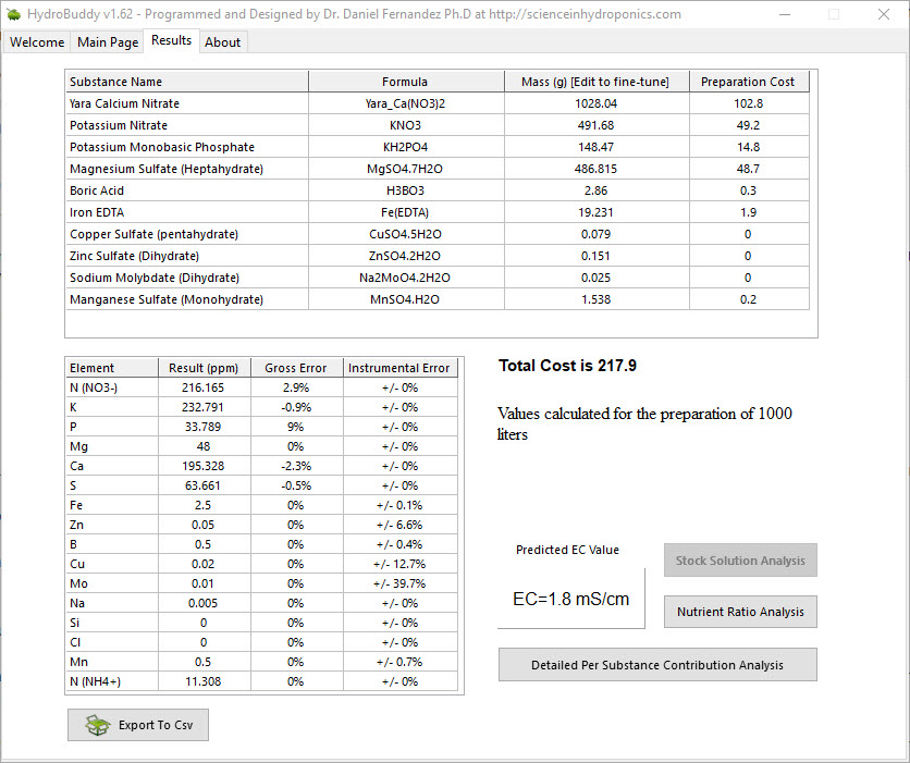
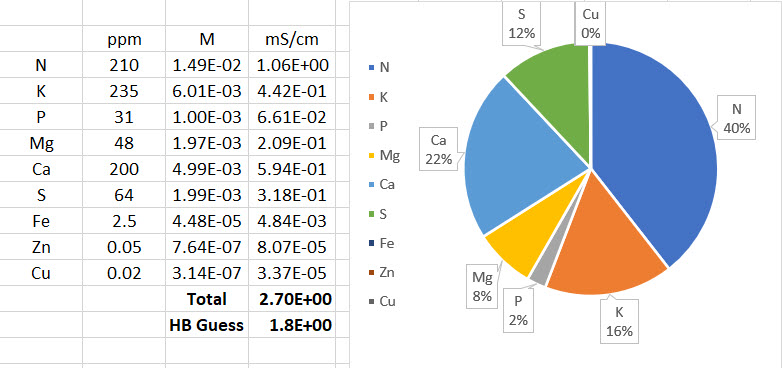
Hydrobuddy’s theoretical conductivity estimates have never been good. As I discussed in a previous post, the program uses a very simple model based on limiting molar conductivities to calculate the EC. The software knows how much each ion conducts when it’s all by itself, so it adds all these conductivity values multiplied by the concentration and assumes there are no additional effects. The conductivity values resulting from this assumption are very large – because there are effects that significantly reduce the conductivity of ions at larger concentrations – so HydroBuddy just cuts the estimation by 35% hoping to reach more accurate values. This works great for some cases, but very badly for others.

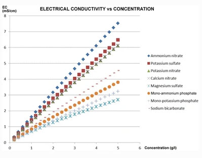
The reason why this happens is that the actual conductivity contribution of some ions decreases more drastically as a function of concentration and due to the presence of other ions compared to others. This means that we need to account for these decreases in conductivity in an ion-specific way. One way to approach this, is to forget about theoretical approximations and just create an empirical model that uses experimental data. This is what I did when I created the empirical model that is present in HydroBuddy from v1.7. This model works really well, provided you are using the exact list of salts that were used to create the model and you stay within the boundaries of concentration values that were used to create it.

This experiment-based solution can be great. It is in fact, a technique I’ve used to create custom versions of HydroBuddy for clients who want to have high accuracy in their EC estimations within the salts that they specifically use. The process is however cumbersome and expensive, my wife and I – both of us chemists – do all the experimentation, and it generally requires an entire day, preparing more than 80+ solutions using high accuracy volumetric material, to get all the experimental data. It is also limited in scope, as any salt change usually requires the preparation of a substantial number of additional solutions to take it into consideration.

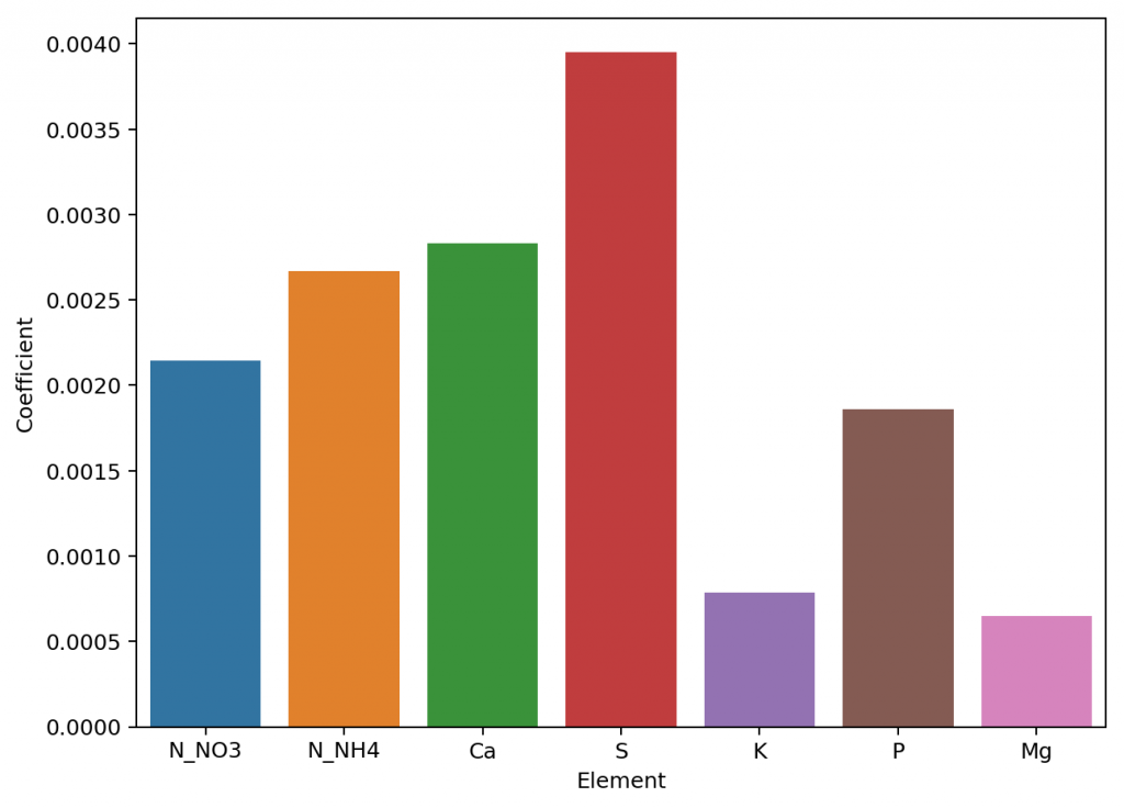
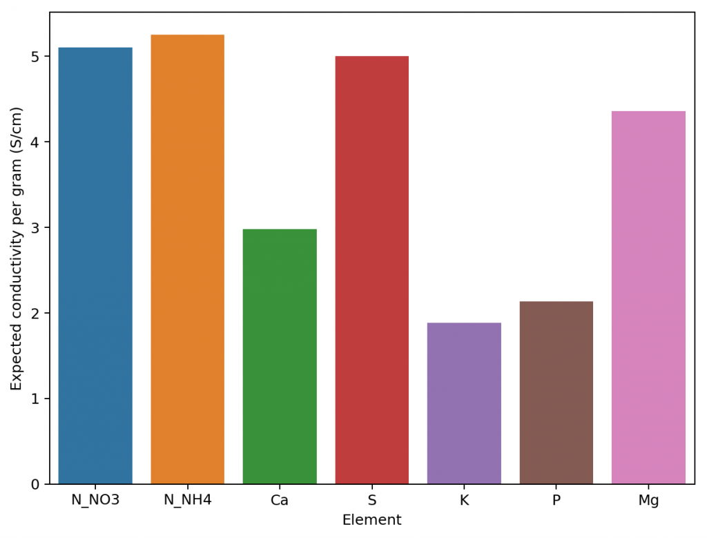
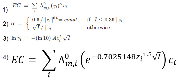
It would certainly be great if we could create a better, fully theoretical, conductivity model. Diving into the literature and programs used for conductivity-related calculations, I found a program called Aqion that implements a more accurate model compared with HydroBuddy’s LMC model. You can read more about their approach here. They use the limiting molar conductivities but introduce additional terms to make ion-specific corrections that are related to both ionic charge and ionic strength. The ionic charge is the electrical charge of each ion, for example, +1 for K⁺ and +2 for Fe⁺², etc. The ionic strength is the sum of the molar concentration of each ion times its charge.

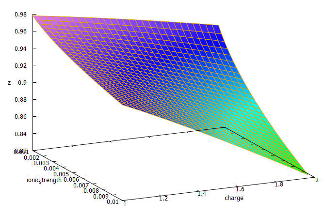
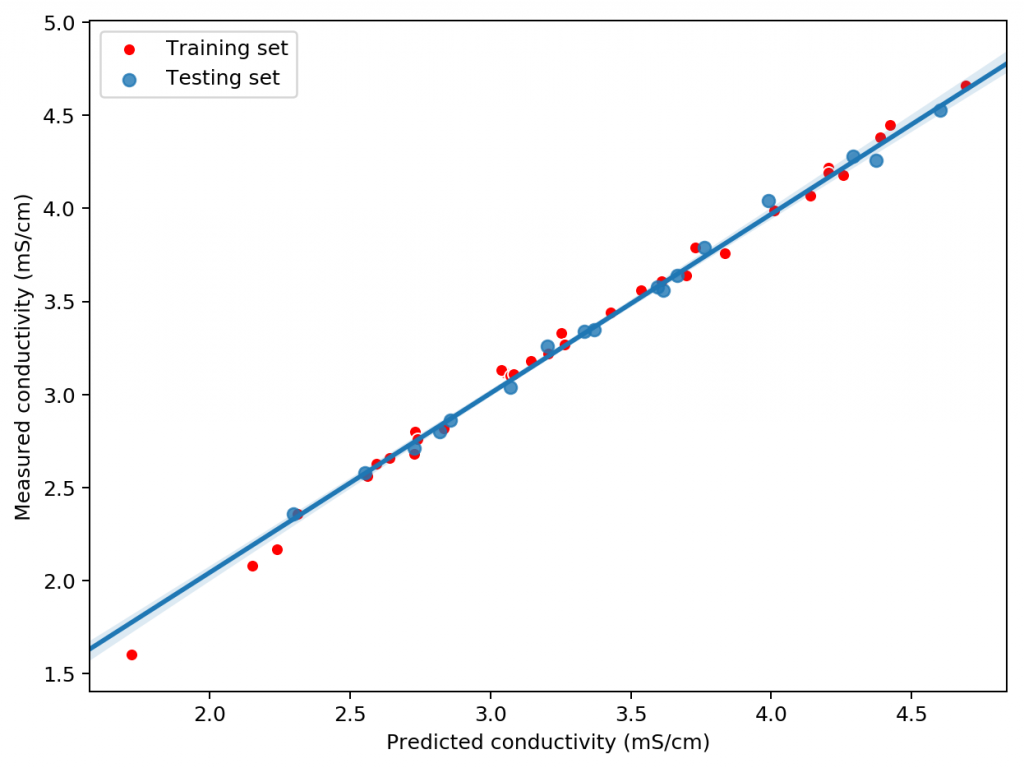
The plot above shows you how this correction factor affects a solution as the ionic strength and charge of the ions change. As a solution gets more diluted, the equation approaches the sum of the conductivities at infinite dilution. Conversely, as the solution becomes more concentrated or the ion charge becomes higher, the drop in the conductivity becomes more pronounced. These are both phenomena that are in-line with experimental observations and much better reflect how conductivity is supposed to change when different ions interact in solution.

The above equation provides us with a more satisfactory theoretical estimation of conductivity compared to the current HydroBuddy LMC model. The new model is able to implement correction factors on a per-ion basis and also changes the magnitude of these corrections depending on how concentrated the solutions are. This new model will be implemented to replace the current LMC model in HydroBuddy v1.9, which will be released in the near future. This should provide significantly more accurate estimates of conductivity for the preparation of hydroponic solutions.

There are multiple open-source projects available online for the creation of pH/EC sensing stations for hydroponics. However, all of the ones I have found use a single Arduino or Raspberry Pi to perform the measurements and store any data, making them unsuitable for applications where more flexibility is needed. For example, a facility using multiple different reservoir tanks for nutrient storage might require multiple pH/EC sensing stations, and single-board wired setups would be unable to accommodate this without a lot of additional development. In this post, I am going to show you a simple pH/EC sensing station I built with an Arduino MKR Wifi 1010 that can communicate with a MyCodo server using the MQTT protocol. Multiple sensing stations could be built and all of them can communicate with the same MyCodo server.

This project makes use of the small pH/EC boards provided by uFire, which have a lower cost compared to those provided by companies like Atlas, but do have adequate electrical isolation to avoid problems in readings when multiple electrodes are put in the same solution. This is a substantial improvement over other low-cost boards where using multiple probes can cause heavy electrical noise and interference. In order to build this project you will require the following materials:

Note, some of the links below are amazon affiliate links. This means that I get a small commission if you purchase through these links at absolutely no extra cost to you. The links to other websites are not affiliate links.

1. Arduino MKR Wifi 1010
2. uFire pH probe
3. uFire EC probe
4. A rugged pH probe with a VNC connector
5. An rugged EC probe with a VNC connector
6. Two Qwiic-to-Qwiic connectors
7. One Qwiic-to-male connector
8. A project box to put everything inside (optional)
9. A micro USB cable

The code for the project is shown below:

#include <uFire_EC.h>
#include <uFire_pH.h>
#include <WiFiNINA.h>
#include <ArduinoMqttClient.h>

#define SECRET_SSID "ENTER WIFI SSID HERE"
#define SECRET_PASS "ENTER WIFI PASSWORD HERE"

//calibration solutions used
#define PH_HIGH_SOLUTION_PH 7.0
#define PH_LOW_SOLUTION_PH  4.0
#define EC_HIGH_SOLUTION_EC 10.0
#define EC_LOW_SOLUTION_EC  1.0
#define CALIBRATION_TEMP    20.0

// topics for the mqtt sensors
// Make sure all stations have different topics
#define EC_TOPIC       "EC1"
#define PH_TOPIC       "PH1"
#define CALIB_TOPIC    "CALIB1"
#define MQTT_BROKER    "ENTER MQTT SERVER IP HERE"
#define MQTT_PORT      1883

int status = WL_IDLE_STATUS;     // the Wifi radio's status
String message;

uFire_pH ph;
uFire_EC ec;
WiFiClient wifiClient;
MqttClient mqttClient(wifiClient);

void check_connection()
{
  if (!mqttClient.connected()) {
    WiFi.end();
    status = WiFi.begin(SECRET_SSID, SECRET_PASS);
    delay(10000);
    if (!mqttClient.connect(MQTT_BROKER, MQTT_PORT)) {
      Serial.print("MQTT connection failed! Error code = ");
      Serial.println(mqttClient.connectError());
      delay(100);
    }
    mqttClient.subscribe(CALIB_TOPIC);
  }
}

void setup()
{
  Serial.begin(9600);
  while (!Serial);

  // connect to wifi and mqtt broker
  check_connection();
  
  // coorectly initialize the uFire sensors
  // note the Wire.begin() statement is critical
  Wire.begin();
  ec.begin();
  ph.begin();
}

void loop()
{
  // mqtt keep alive
  mqttClient.poll();

  // read messages 
  message = "";
  while (mqttClient.available()) {
      message += (char)mqttClient.read();    
    }

  // execute calibration if requested
  Serial.println(message);
  if (message == "EC1_HIGH") ec.calibrateProbeHigh(EC_HIGH_SOLUTION_EC, CALIBRATION_TEMP);
  if (message == "EC1_LOW")  ec.calibrateProbeLow(EC_LOW_SOLUTION_EC, CALIBRATION_TEMP);
  if (message == "PH1_HIGH") ph.calibrateProbeHigh(PH_HIGH_SOLUTION_PH);
  if (message == "PH1_LOW") ph.calibrateProbeLow(PH_LOW_SOLUTION_PH);

  // Measure EC 
  ec.measureEC();
  Serial.println((String) "mS/cm: " + ec.mS);

  // Measure pH
  ph.measurepH();  
  Serial.println((String) "pH: " + ph.pH);

  // Ensure the wifi and mqtt connections are alive
  check_connection();

  // post EC to MQTT server
  mqttClient.beginMessage(EC_TOPIC);
  mqttClient.print(ec.mS);
  mqttClient.endMessage();

  // post pH to MQTT server
  mqttClient.beginMessage(PH_TOPIC);
  mqttClient.print(ph.pH);
  mqttClient.endMessage();

  // ensure sensors are not probed too frequently
  delay(1000);

}

Once you get all the materials you should first assemble the components. Connect the pH and EC board together using the Qwiic-to-Qwiic connector, then use the Qwiic-to-male connector to hook up one of these boards to the Arduino (doesn’t matter which one). Connect the black cable to ground, red cable to 5V, blue cable to SDA, and yellow cable to SCL. Set up your board according to the instructions in the Arduino MKR wifi 1010 getting started page, modify the code above to properly include information about your wifi network, calibration solutions, and MQTT server, then upload the code. The Arduino will connect to your Wifi and MQTT servers and automatically reconnect when there are connection issues.

The above code will also post the readings of the pH and EC sensors to topics PH1 and EC1 respectively if you add an input in MyCodo to capture these readings you should be able to store them and take control actions using the MyCodo interface. Additionally, the Arduino code will respond to calibration requests published to the topic “CALIB1”. For example, if you want to calibrate your EC sensor with a two-point calibration method with a standard solution with an EC of 10mS/cm, you would put the electrode in the calibration solution, then send the message “EC1_HIGH” to the CALIB1 topic and the Arduino will perform the task as requested. The code assumes you will want to do 2 point calibrations for both EC and pH, with the calibration events triggered by EC1_HIGH, EC1_LOW, PH1_HIGH, and PH1_LOW. Note that the definition of the EC and pH values of the calibration solutions should be changed to the solutions you will be using within the code. The high/low values in the code, as is, are 10mS/cm|1mS/cm for EC and 7|4 for pH.

On my previous post you can read about how I ran experiments to develop a conductivity model using empirical data in order to improve our ability to predict EC values from the concentration of individual nutrients in a hydroponic nutrient solution. In this post I will now talk about how this was finally implemented in HydroBuddy, what form it took and what kind of result can be expected from it. The implementation discussed in this post has already been updated to the HydroBuddy github along with all the experimental data used to derive this empirical EC model.

Given the amount of data and the nature of the problem at hand, the easiest and most accurate way to build a model was to use a simple linear regression algorithm. As previously shown this model was able to give great results within the data, even when performing random training and testing splits. I have added a jupyter notebook to the github repository, along with all the data we measured in order to allow you to see how all the calculations were done, how the model was created and the sort of accuracy the model got within the set of experimental results. You can also play with this notebook to develop your own models or analyse the data any further if you wish. You can also try to reproduce our experiments and help verify our results. The linear model was translated into FreePascal and added to HydroBuddy although the program still retains the ability to estimate conductivity using the previously available LMC based model.

The fact that we were able to create a model to accurately determine conductivity within this experimental space does not mean that this model will work to magically determine the conductivity of any hydroponic formulation. These experiments were designed using five salts – calcium ammonium nitrate, ammonium sulfate, potassium sulfate, magnesium sulfate and monopotassium phosphate – which means that although our model is able to greatly describe conductivity in this space, the model is likely to run into trouble when attempting to describe a space that deviates too strongly from the one described above. This will be most evident whenever there are some cations or anions that are not present at all within these experiments. For example when silicates, chlorides or other such salts are used or when strong acids or bases are added to the solution.

Another important issue is the way these ions are paired. In our experimental process the concentration of Ca and N as nitrate always increased at the same time, meaning that the linear model implicitly carries this assumption. A setup were magnesium nitrate or potassium nitrate are used as well, will contain deviations from the current model that it is likely not very well prepared to deal with. A similar problem might happen when salts such as ammonium monobasic phosphate are used, since our model only contained a single example of a phosphate salt (monopotassium phosphate). While it is not easy to predict how much accuracy will be lost in these cases, we do expect the model to be significantly more inaccurate as other salts are used.

Additionally, our experimental setup did not contain any corrections of pH values, so the conductivity values described include a pH drift related with the amount of acid contributed by the potassium monobasic phosphate, which was not neutralized by a base. This will also cause differences with conductivity, if the conductivity is measured after the pH of the solution is corrected to the proper range used within the hydroponic process. Although at the concentration values used in hydroponics this should not be a big issue, it is still something worth considering.

As I mentioned above, the model is already implemented within the github repository – if you want to compile the program yourself – but the binaries won’t be updated to v1.8 until later this week. I look forward to your feedback about the model and hope it can help – at least some of you – to dramatically improve the estimations of conductivity of your hydroponic nutrient solutions.

Electrical conductivity (EC) is one of the most useful parameters in the practical preparation of hydroponic nutrient solutions. This is because knowing the expected conductivity of a nutrient solution can allow you to prepare solutions without having to measure the total volume exactly, a parameter that is often hard to accurately determine in practice. Although determining the target conductivity is easy to do using small preparation volumes – which can be done accurately – it is often impractical to do so routinely, which is necessary if the actual composition of the nutrient solution is being changed as a function of time. Due to all the above, it is important to come up with accurate models to estimate the EC of nutrient solutions with only information about their mineral composition, without having to measure the value experimentally. In this post I am going to talk about how I created a model to do exactly this, taking advantage of multi-variable experimentation and simple modeling techniques.

The problem with conductivity modeling is that not all salts contribute the same to the conductivity of a nutrient solution. For example potassium sulfate can contribute significantly more to conductivity per gram compared to a salt like monopotassium phosphate. Furthermore, the addition of some salts can affect the conductivity of others (see my previous post on conductivity modeling in Hydrobuddy for more details). In the regime we use in hydroponics, the determination of electrical conductivity using data from limiting molar conductivity can lead to very skewed results, which makes these estimations of little usage in practice.

To solve this issue, I designed an experiment where 50 different EC measurements were made for different hydroponic nutrient solutions within the range of concentrations of nutrients that are reasonably expected in hydroponic culture, with some values being above these in order to ensure that all values encountered in practice will be within the measured ranges. The image above shows you all the concentrations that were measured within the experiment. To prepare the solutions I used calcium ammonium nitrate, potassium sulfate, magnesium sulfate heptahydrate, monopotassium phosphate and ammonium sulfate. All of these were agricultural grade salts in order to reflect the same impurities expected in a normal hydroponic setup. Note that no heavy metal salts were used since their contribution to the EC of a hydroponic nutrient solution is negligible.

Concentrated solutions of all the salts were prepared in 250mL volumetric flasks using a +/-0.001g scale and aliquots of these solutions were drawn using 5mL plastic syringes (+/- 5%) in order to prepare final 250mL solutions using volumetric flasks. Conductivity measurements were done using an Apera EC60 conductivity meter that was previously calibrated using a 2 point calibration method. All the solutions were prepared using distilled water. The target concentrations for the solutions were determined using a pseudo random number generator in order to try to ensure a random distribution of samples within the concentration space of interest.

Using this data we constructed a linear model to attempt to predict conductivity. In order to evaluate the model we randomly split the results to get 33 data points used for model construction and 17 points left for model validation. Performing this process 100 times shows that the mean R2 of the model on the training set is 0.995 while the average on the training set is 0.994. This shows that the model is able to properly generalize the conductivity data in order to properly predict the conductivity of the solution across the space studied. The mean absolute error in the testing set was 0.036 mS/cm. This shows the high certainty with which we can make conductivity predictions.

Exploring the model coefficients can also show us how different the contributions of the different elements to the conductivity of the nutrient solution can actually be. These results are surprising if you compare them to the conductivity contributions per gram that are expected from the limiting molar conductivity values, which are the conductivity values the ions exhibit on their own under very high dilutions (this is also the method used in HydroBuddy <=v1.65). We can clearly see here that in reality we are getting way more conductivity out of sulfate compared to the other elements and significantly less from magnesium. This means that at the makeup and concentration values used in hydroponics the Mg ions are not being able to contribute as much as they can when they are alone because their activity is being lowered by the other ions in solution, while the opposite case applies to sulfate.

The above shows us why conductivity in hydroponics is so complicated, it shows how ions do not contribute equally to conductivity and how they behave very differently in real hydroponic solutions. Thankfully the above also shows how we can create a model using experimental data that is actually able to predict conductivity, since the relationships – although different than expected – are still highly predictable when enough experimental data is available. All the above experimentation took 4 hours to do – with the help of my lovely wife, who is also a chemist – and should allow me to add a very powerful model to predict hydroponic nutrient solution EC values to HydroBuddy.

All the above experimentation data will be open source and available in a github repository soon. We also hope to show you how all of this was done in a youtube video in the near future.

Electrical conductivity is a very commonly used measurement in hydroponics, yet a very poorly understood one. I have written several posts about conductivity in the past (1,2,3) and today I want to talk about the use of the term “Total Dissolved Solids” and the poor usage of the unit “ppm” in order to express a measurement of electrical conductivity. In this article I will walk you through why this term exists in the first place and why its use in hydroponics is terribly misleading for growers.

Conductivity is just a measure of how easy it is for an electrical charge to go from one electrode of a certain area to another. It’s generally expressed in mS/cm, which is a measurement of conductance (the opposite of resistance) and area (the area of the electrode). How in the world do we get from this to a measurement like “ppm”, which measures the concentration of something in mg/L? What does a measurement of 500 ppm even mean? What is it that we are expressing a concentration of?

The answer lies in the practical uses of conductivity and a simplification to make the evaluation of water sources easier. Conductivity is generally linearly proportional to the amount of a pure salt dissolved in solution at low concentrations. For a pure salt like table salt (NaCl) the higher the concentration of the salt in solution the higher the conductivity (you can see this in the image above). People working on water quality realized that they generally dealt with similar salt combinations (Mg and Ca carbonates and possibly some Na and K chlorides) so they decided to use some standard salt mixtures (say KCl, NaCl or some mixture of Ca/Mg/K/Na salts) and then use conductivity as a proxy for the concentration of these things that are actually in solution. So the “ppm” that your EC meter reads is just the equivalent conductivity of some standard. A meter reading 500 ppm in conductivity is telling you “your solution has the same conductivity as a solution of the standard at 500 ppm”. The “standard” can change – as mentioned before – which is why there are several different TDS scales. One meter might be telling you it’s the same conductivity as a solution of KCl with that concentration, while another might be in NaCl.

The above is very useful when you’re measuring things that tend to be similar but this becomes a complete nightmare when the composition of what you’re measuring can change substantially. In hydroponics you have a wide variety of different salts, all with very different conductivity values at different concentrations. Look at the graph above, which shows the conductivity as a function of concentration for 8 different salts commonly used in hydroponic culture. If you prepare three solutions, one with 1000 ppm solution of potassium sulfate, another with 1000 ppm of monopotassium phosphate and another with 1000 ppm of ammonium nitrate and measure them with your conductivity meter they would all give very different results. The meter might be close to 0.95mS/cm for the monopotassium phosphate, but it might read almost 1.5 mS/cm for the potassium sulfate. Both solutions have 1000 ppm of “total dissolved solids” but the conductivity meter is telling you one has 500 ppm and the other almost 800 ppm, none of them even close. This is because “total dissolved solids”, as used in water quality measurements, is a meaningless measurement in hydroponics as it relates to the actual ppm values of things dissolved.

This is the main reason why you should never compare the EC values of nutrients that contain different ratios of salts, because they are simply not the same. One nutrient might give you 100 ppm of potassium at some EC level, while another might give you 200 ppm. Thinking that having the same EC level means that both are at the same “strength” is a big mistake, since this is never going to be the case when two nutrient solutions are mixed with different ratios of nutrients. This is also why comparing vegetative and bloom formulation EC values is not correct. A solution in veg might contain a lot more of nitrates while a solution in bloom might contain more phosphates. As we saw above this might mean that a solution of the “same strength” might actually have a significantly lower measured EC value.

Since the TDS measurement is not telling you anything about “total dissolved solids” in hydroponics, you should avoid using it to avoid confusion. This is important since nutrient concentrations are usually expressed in ppm as well, ppm of actual nutrients dissolved in solutions. Instead use the normal conductivity measurements of your meter in conductance per area. You should also take care to only use EC values to talk about comparative strength when you’re talking about a formulation where the ratios of nutrients remain the same. If that’s not the case, then you should not talk in comparative terms between the two solutions as this might deviate a lot from reality.

My advice is to not think in EC terms to begin with, but to think about nutrient concentrations, prepare solutions that match the concentrations you want and then use the EC of those solutions as references to know whether they are prepared correctly or not. The conductivity should be a measurement used for confirmation but not as a guiding principle. For example the aim should be to “prepare a solution containing 150 ppm of N and an K:N ratio of 1.2” not to “prepare a solution with an EC of 1.2 mS/cm”.

People who use Hydrobuddy can be confused by its conductivity estimates, especially because its values can often mismatch the readings of conductivity meters in real life. This confusion can stem from a lack of understanding of how these values are calculated and the approximations and assumptions that are made in the process. In this post I want to talk about theoretically calculating conductivity, what the meters read and why Hydrobuddy’s estimations can deviate from actual measurements.

The images above show the use of HydroBuddy for the calculation of a standard Hoagland solution for a 1000L reservoir. The Hoagland solution’s recipe is expressed as a series of elemental concentrations, all of them in parts per million (ppm) units. The results show that the final conductivity of this solution should be 1.8 mS/cm but in reality the conductivity of a freshly prepared full strength Hoagland solution will be closed to 2.5mS/cm. You will notice that HydroBuddy failed to properly calculate this value by an important margin, missing the mark by almost 30%. But how does HydroBuddy calculate this value in the first place?

Conductivity cannot be calculated by using the amount of dissolved solids in terms of mass because charges are transported per ion and not per gram of substance. To perform a conductivity calculation we first need to convert our elemental values to molar quantities and then associate these values with the limiting molar conductivity of each ion, because each ion can transport charge differently (you can find the values HydroBuddy uses in the table available in this article). This basically means we’re finding out how many ions we have of each kind and multiplying that amount by the amount each ion can usually transport if it were by itself in solution. The sum is the first estimate in the calculation of conductivity.

The image above shows the result of these calculations for an example with a perfectly prepared Hoagland solution. You can see that the estimate from limiting molar conductivity is initially 2.7 ms/cm – much closer to the expected 2.5 mS/cm – but then HydroBuddy makes an additional adjustment that lowers this down to 1.8 mS/cm. This is done because limiting molar conductivity values make the assumption of infinite dilution – what the ion conducts if it were all by itself in solution – but in reality the presence of other ions can decrease the actual conductivity things have in solution. HydroBuddy accounts for this very bluntly, by multiplying the result by 0.66, in effect assuming that the measured value of conductivity will be 66% of the value calculated from the limiting molar conductivity values. This is of course wrong in many cases, because the reduction in activity due to the presence of other ions is not as strong. However it can also be correct in many cases, primarily depending on the substances that are used to prepare the formulations and the ratios between the different nutrients.

In my experience HydroBuddy tends to heavily underestimate the conductivity of solutions that receive most of their conductivity from nitrates, as this example, but it tends to do much better when there are large contributions from sulfate ions. When I first coded HydroBuddy all my experiments were being done with much more sulfate heavy solutions, so the correction parameter value I ended up using for the program ended up being a bad compromise for solutions that deviated significantly from this composition. With enough data it might be possible to come up with a more advanced solution to conductivity estimations in the future that can adjust for non-linear relationships in the conductivity and activity relationships of different ions in solution.

If your measured conductivity deviates from the conductivity calculated in HydroBuddy you should not worry about it, as HydroBuddy’s values is meant to be only a rough estimate to give you an idea of what the conductivity might be like but, because of its simplicity, cannot provide a more accurate value at the moment. The most important thing is to ensure that all the salts, weights and volumes were adequately measured in order to arrive at the desired solution.

Conductivity is perhaps the most misunderstood and erroneously used measurement in hydroponic culture. This has a lot to do with conductivity also being called a “totally dissolved solid” (TDS) measurement and the conductivity scale being expressed in “ppm” units, concentration units which only cause confusion in this area. Today I want to talk about an important consequence of this confusion that happens when you try to compare the conductivity of different nutrient solutions. I’ll talk about a recent case I encountered and how it generated significant problems due to a natural misunderstanding of how conductivity works.

–

–

A grower wanted to run a side by side trial of two nutrient formulations using identical growing conditions. This grower then decided that the best way to do this was to ensure that the conductivity and pH of the two solutions were identical after preparing the nutrient solutions, then they would both be equivalent in terms of their strength and differences in results would be entirely due to the differences in ionic ratios between both of them. The media was the same, the environment was the same and plant genetics were the same.

However there was a small problem with this thinking. The same conductivity across two different solutions is not the same thing. You might think that using a conductivity of 2.0 mS/cm across two different nutrient solutions might mean that their “strength” is the same, but in reality the strength of a solution – as per what a plant really experiences – is determined by its osmotic pressure and osmotic pressure – although proportional to conductivity within the same solution – cannot be extrapolated when the composition of the solution changes. This confusion is further expanded when people see the conductivity numbers in ppm because the expression in mg/L makes them think there is the same “amount of stuff” in the two solutions. This is not the case.

All the ppm does is tell you that your solution has the same conductivity as a reference with that ppm concentration (commonly NaCl or KCl) but it tells you nothing about how many dissolved solids are really present within your nutrient solution. Given that non-conductive substances also affect the osmotic pressure of a solution it can happen that a nutrient solution with the same conductivity as another one in reality has a lot more dissolved solids, making it far more concentrated in real terms compared to the other one.

–

–

In the above mentioned particular case one solution had a chelating agent that effectively made a significant number of ions neutral in charge (effectively making them non-conductive) reducing the measured conductivity by around 20% at the same osmotic pressure as the other solution. So while the grower was feeding the two solutions at the exact same conductivity, the second solution was around 20% more concentrated in real terms – osmotic pressure terms – compared to the other one. Plants responded very negatively to this – as the conductivity was already quite high – so the grower erroneously assumed that this was due to the ionic ratios instead of it simply being due to an error in judging concentrations. The second solution was a lot stronger in real terms, although the conductivity was the same.

When comparing two nutrient solutions you should therefore resort to measurements different than conductivity because the conductivity of two different solutions with different ion compositions cannot be compared, the same level of conductivity will result in two completely different osmotic pressure values. Their strengths will not be the same. If you want to compare two different solutions at the same real strength then you need to use an osmometer to determine this point and sadly osmometers are neither cheap nor practical to use.

However another possibility is to simply compare at a constant concentration of a given element. Have a lab analysis of the two fertilizers made – remember you cannot trust labels to give you the real composition values – calculate how much of a given element, for example N, is present at a given application rate and then dial in the other fertilizer to match that N concentration. The osmotic pressures will probably be different but at least under this sort of A/B test you will be comparing apples to apples in the sense that the only variable will be the N:X ionic ratios between the two solutions. Total strengths will differ but this will be due to differences in ionic ratios, which is probably what you want to test.