What is water hardness?

There are many parameters that determine the quality of a water source. Water that has a composition closer to distilled water is considered of a higher quality, while water with many dissolved solids or high turbidity is considered low quality. Calcium carbonate, magnesium carbonate, calcium sulfate and calcium silicate are some of the most common minerals that get dissolved into water as it runs through river beds and underground aquifers. The carbonates and silicates will make water more basic, will increase the water’s buffering capacity and will also increase the amount of magnesium and calcium present in the water.

Water hardness is determined experimentally by measuring the amount of Calcium and Magnesium in solution using a colorimetric titration with EDTA. Although both Calcium hardness (specific amount of Ca) and Magnesium hardness (specific amount of Mg) are measured, total water hardness (the sum of both) is the usually reported value. The result is often expressed as mg/L of CaCO₃, telling us how much CaCO₃ we would require to get a solution that gave the same result in the EDTA titration.

The Calcium and Magnesium present in water sources with high hardness is fully available to plants – once the pH is reduced to the pH used in hydroponics – and it is therefore critical to take these into account when formulating nutrients using these water sources. It is a common myth that these Ca and Mg are unavailable, this is not true.

What about alkalinity?

Water alkalinity tells us the equivalent amount of calcium carbonate we would need to add to distilled water, to get water that has the same pH and buffering capacity. An alkalinity value of 100 mg/L of CaCO₃ does not mean that the water has this amount of carbonate, but it means that the water behaves with some of the chemical properties of a solution containing 100mg/L of CaCO₃. In this particular case, it means that the water requires the same amount of acid to be titrated as a solution that has 100mg/L of CaCO₃.

Water sources with high hardness will also tend to have high alkalinity as the main salts that dissolve in the water are magnesium and calcium carbonates. Since these carbonates need to be neutralized to create a hydroponic solution suitable to plants, the anion contribution of the acid that we will use to perform the neutralization needs to be accounted for by the nutrient formulation.

An example using Valencia, Spain

Valencia, in the Mediterranean Spanish coast (my current home), has particularly bad water. Its water has both high alkalinity and high hardness, complicating its use in hydroponics. You can see some of the characteristics of the water below (taken from this analysis):

Hard water creates several problems. Since Calcium nitrate is one of the most common sources of Nitrogen used in hydroponics, how can we avoid using Ca nitrate? Since we have more than enough. Also, how can we neutralize the input water so that we can make effective use of all the nutrients in it without overly increasing any nutrient, like P, N or S, by using too much of some mineral acids?

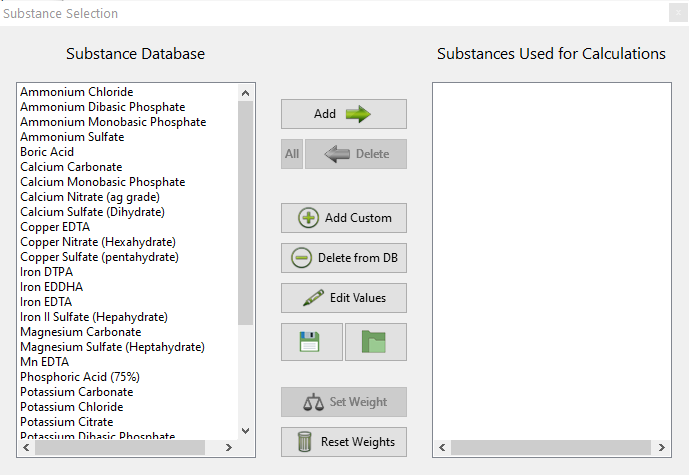
Creating a one-part solution for very hard water

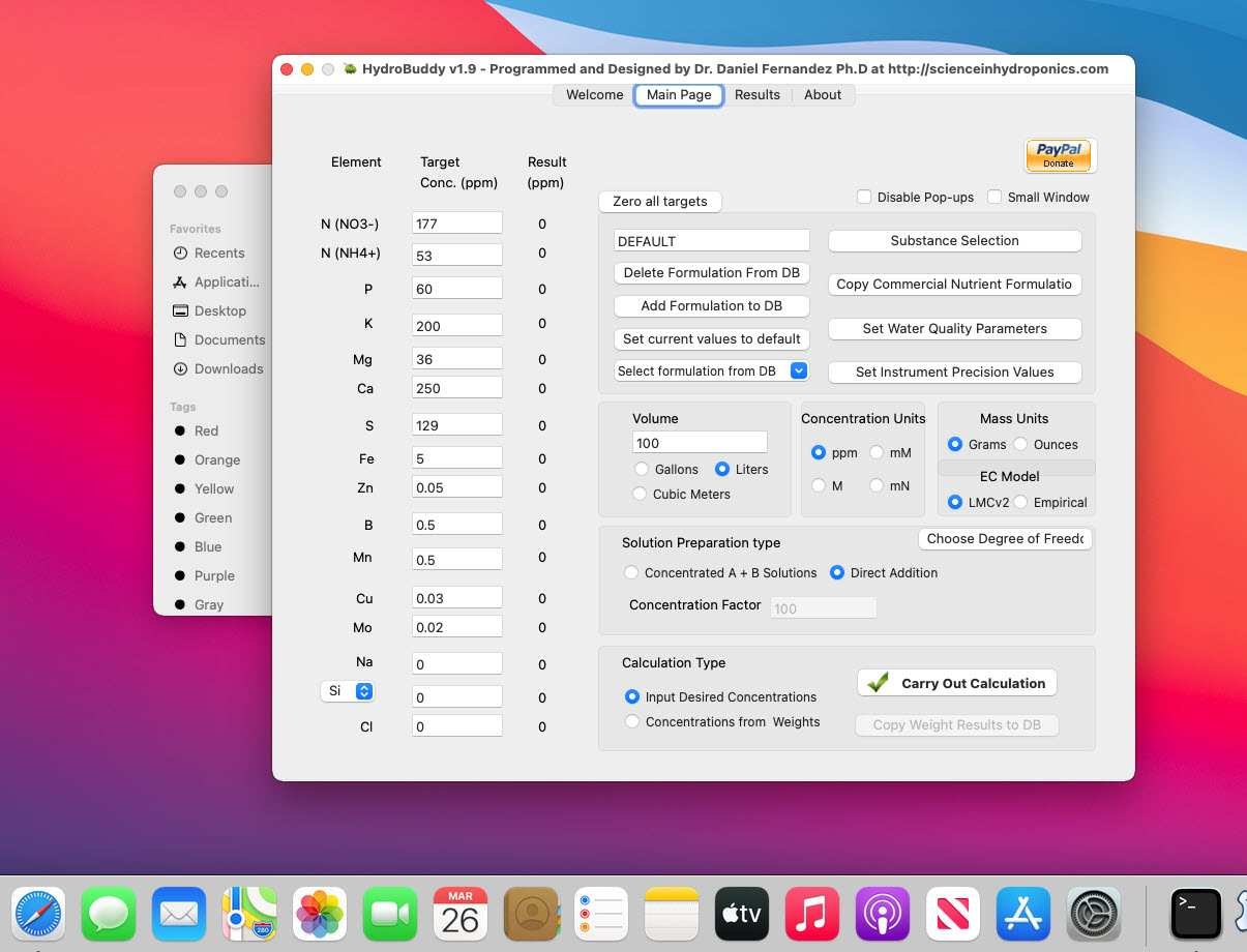
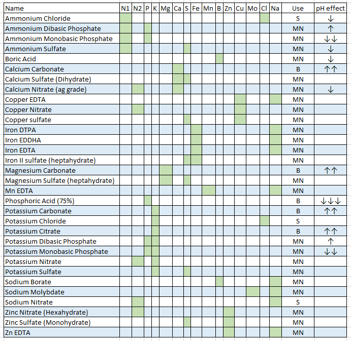
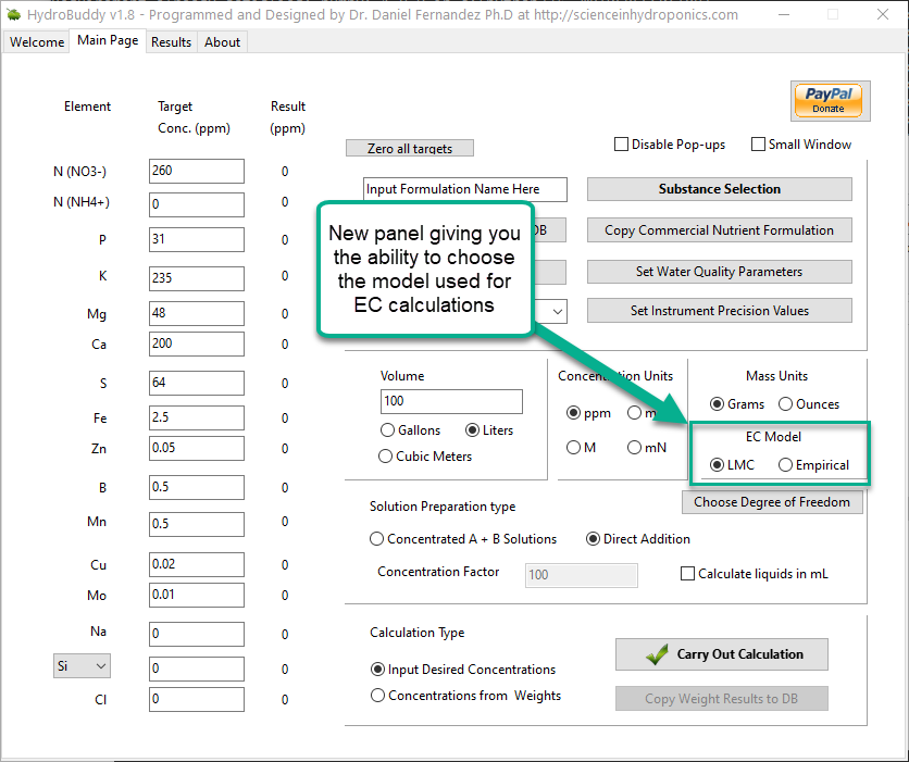
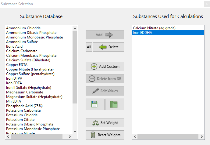
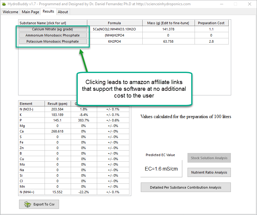
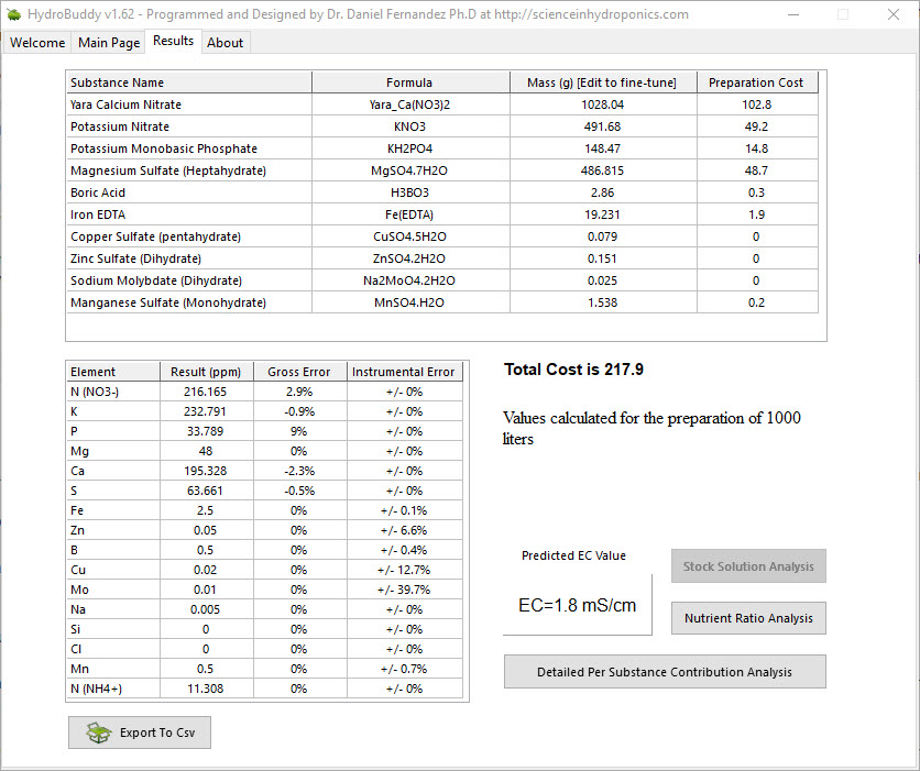
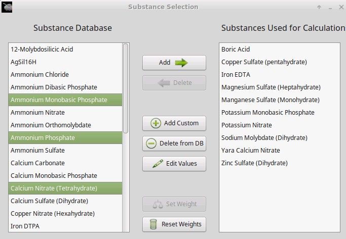
HydroBuddy allows us to input the characteristics of the input water into the program so that we can work around them while designing nutrient solutions. To get around the above mentioned problems – but still ensure I could easily buy all the required chemicals – I decided to use a list of commonly available fertilizers. I used Calcium Nitrate, Magnesium Nitrate, Potassium Nitrate, Phosphoric acid (85%) and a micro nutrient mix called Force Mix Eco (to simplify the mixing process). This micronutrient mix is only available to people in the EU.

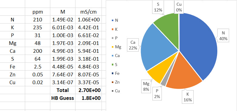
Note that we use absolutely no phosphates or sulfates, since the solution already contains more than enough sulfur (89 ppm) and we need to add all the Phosphorus as phosphoric acid to be able to lower the alkalinity. I determined the amount of P to add by setting P to zero, then using the “Adjust Alkalinity” to remove half of the alkalinity of the water using phosphoric acid. This is more than enough P to be sufficient for higher plants. The above nutrient ratios should be adequate for the growth of a large variety of plants, although they are a compromise and not ideal for any particular type of plant.

Since we are adding no sulfates and the pH of the solution is going to be very low (because of the phosphoric acid), we can add all of these chemicals to the same solution (no need to make A and B solutions). The values in the image above are for the preparation of 1 gallon of concentrated solution. This solution is then added to the water at 38mL/gal of tap water to create the final hydroponic solution.

Does it work?

I have experimentally prepared the above concentrated solution – which yields a completely transparent solution – and have created hydroponic solutions I am now using to feed my home garden plants. After adding to my tap water – initial pH of 7.6 – I end up with a solution at a pH of 5.6-5.8 with around 1.5-1.8mS/cm of electrical conductivity. The plants I’m currently growing – basil, rosemary, chives, mint, malabar spinach and spear mint – all seem to thrive with the above solution. I am yet to try it on any fruiting crops, that might be something to try next year!

Are you growing using hard water, have you prepared a similar one-part for your hard-water needs? Let us know what you think in the comments below!

Tissue Analysis

To grow great plants, we need to grow plants that have a healthy mineral composition. Although there are no theoretically established values for what the mineral composition of a plant should look like, we have grown healthy plants and have established, through analysis of their tissue, what this mineral composition should empirically be. By sampling the leaf tissue from your plants and sending it to a lab for analysis, you can know what the composition of your tissue is and how it compares to healthy plants grown by others.

The question is, can we create a nutrient formulation just from the tissue composition we want to get?

Nutrient solution targets from tissue analysis

Turns out, you can figure out the elemental concentrations that are required in solution to get to certain concentrations in tissue. My colleague and friend – Bruce Bugbee – proposed in this paper about nutrient management in 2004 how this could be done. To achieve this, we make the assumption that all elements taken up by the plant will be deposited as minerals upon transpiration – because minerals cannot leave the plant as gases – so knowing the amount of water that will transpired per amount of tissue grown, we can figure out how much of that element needs to be in the water.

The volume of water required to grow a certain mass of tissue is called Water Use Efficiency (WUE). It is expressed as gram of tissue per liter of water transpired and has values from 3.0 to 6.0. Higher WUE values imply the plant is growing more efficiently, requires less water to grow the same mass of tissue, while a lower WUE implies the plant is less efficient and needs to transpire more to grow. Conditions that increase growing efficiency and decrease transpiration, such as carbon dioxide enrichment and high humidity, tend to increase WUE, while conditions that create inefficient growing – like low humidity with high temperature – tend to decrease it.

If we grow plants with a solution where we determine the nutrients according to the WUE and the concentrations in tissue we want, we can create very effective solutions that lower the probability of over accumulation of nutrients in the root zone and the solution. This allows for solutions that require no dumping and create very healthy plants in recirculating systems (for which Deep Water Culture, DWC, is the most common example).

Doing this process in HydroBuddy

From v1.99, HydroBuddy now includes a “Tissue Analysis” dialogue that allows you to use target tissue concentrations and a certain WUE value, to figure out what the required nutrient concentrations in a hydroponic solution would be like. The program also includes a small Database with tissue targets for certain plants and certain stages of development. There are also a couple of links that point you to resources where you can find a wide variety of different plant species and development stages if the ones that interest you are not included in the software’s default DB configuration.

The image below shows you an example where I determined the target solution concentrations required to grow a tomato plant that has the composition expected for a tomato plant in early flower.

How do I figure out the WUE?

As you can see, the above process requires you to input the WUE. This ranges from 3 to 6. It is not easy to measure in the environment, so the best practical solution is to assume your WUE is about 3.5 (the default value), prepare solutions with those concentrations and then observe how the EC of the solution changes as a function of time.

A solution that is prepared with a concentration that would be appropriate for the exact WUE of the plants will have an initial decrease in EC – as nutrients that are taken actively are rapidly taken up – followed by more stable to slightly decreasing EC conditions as uptake changes to be mostly passive. This cycle is repeated when solution is replenished to recover the initial volume in a recirculating system. A solution that is prepared too concentrated will have an increasing EC while a solution that is prepared too diluted will show a consistently decreasing EC. If your EC decreases more sharply with time then you need to assume a higher WUE, if your EC increases then you need to lower your WUE assumption.

Limits of the approach

While this approach can be very useful to create long lasting solutions, especially in recirculating systems, it suffers from some important limitations.

The first is that it doesn’t account for changes in uptake due to changes in pH or availability in solution. This is the reason why the recommendations for elements like Fe and Mn, might be significantly lower than what you commonly see in nutrient solutions. In the above example, the solution requires only around 0.35ppm of Fe, but this means we need 0.35ppm of fully available Fe for the plant, which in reality might mean having 1.5ppm of Fe or more of added Fe, depending on the chemical form of Fe and the pH of the solution.

The above implies that values should not be used without considering the context and that this context might be much more important for some nutrients, for example micro nutrients, than for other elements, for example K and Ca, for which the availability windows and plant uptake are much more straightforward. The plant characteristics should also be taken into account. While a leaf tissue derived approach might only require 50 ppm of Ca in a lettuce crop, we know we need to feed more due to the poor water transport of this plant into new leaves.

Second, the approach assumes that all we care about is leaf composition. This is a perfectly fine if we are growing leafy greens, but if you’re growing a tomato plant, the composition will be heavily split between leaves and fruits as soon as flower pollination ends. For this reason, the nutritional needs of other important tissues – such as sink organs – should be considered very carefully when following this approach. In the case of tomatoes, this might mean feeding substantially higher levels of K, as this element has a much higher concentration in fruits than it has in leaves.

Crops that have changing nutritional needs due to changes in the composition of the tissue formed, require different nutrient solutions as a function of time, as we need to match the overall expected composition of the entire plant, not just the leaves.

Conclusions

Nutrient formulations do not need to be just trial and error. Up until now, besides a formulation database, HydroBuddy had no feature to help growers create formulations with any scientific basis. This new feature, introduces the ability to use target leaf tissue composition and WUE as a way to guide the initial formulation of nutrient solutions. While you still need experience to figure out when to overrule these values and increase or decrease concentrations, it does provide basic blue prints to build from. An analysis of how a formulation derived from tissue compares with your current formulation might also give you some insights into whether you are over or under feeding any elements.

Have you use the HydroBuddy’s leaf tissue analysis feature? Leave us some comments below!

Today I am releasing a new version of HydroBuddy (v1.9) which contains many suggested and needed improvements from the previous version of the software. In this post I want to discuss the changes within this release and how they will affect the way things are done in the program. Some big changes have been implemented so make sure you go through the list below if you want to use this new version. Thanks to all of you who contributed your suggestions about HydroBuddy and/or reported bugs to me.

Here is the list of changes in this version:

• A MacOS binary compiled in Big Sur 11.0.1 has been released.
• Ability to make any formulation the “default” formulation. This selected formulation is loaded when the software is started.
• The LMC conductivity model has now been replaced with LMCv2 which is an important improvement. See here to learn more. The LMCv2 model now adjusts conductivity based on each specific ion’s charge and the overall ionic strength of the solution. It now includes no arbitrary terms.
• The treatment of liquids/solids in the program has now been changed. Instead of specifying liquid or solid (and the program having to make assumptions) users can now select whether the percentages and substance amounts are going to be either in g and w/w% or in mL and w/v%. This should simplify the interpretation of results and the addition of substances.
• An additional column has now been added in the results page to specify the unit of the amount being calculated. When a user wants a substance’s contribution to be calculated in mL, the appropriate unit will be shown here.
• When adding a new substance, all fields are reset to null values (previously the program kept the values from previously opened/updated substances).
• Density has now been eliminated as a variable used in the program since it is not needed if there is no cross between w/w% and w/v% calculations. It is only kept in the “Copy commercial nutrient formulation” dialogue.
• An error where P and K were mixed up in the product comparison window of the “Copy commercial nutrient formulation” function has now been fixed.
• The wording of options in the “Substance selection” dialogue has been changed so that the buttons better describe what they do. For example the “Delete” button has now been changed to “Do not use”.
• Two buttons have been added next to the EC model prediction in order to allow users to increase or decrease the EC by adjusting all nutrient concentrations by +5%/-5%. This will allow you to see how nutrient concentration changes affect conductivity in a straightforward manner.

The above modifications are now committed to the github repository as well. Feel free to take a look if you’re interested in how any of the above variations were coded into the program.

Hydrobuddy’s theoretical conductivity estimates have never been good. As I discussed in a previous post, the program uses a very simple model based on limiting molar conductivities to calculate the EC. The software knows how much each ion conducts when it’s all by itself, so it adds all these conductivity values multiplied by the concentration and assumes there are no additional effects. The conductivity values resulting from this assumption are very large – because there are effects that significantly reduce the conductivity of ions at larger concentrations – so HydroBuddy just cuts the estimation by 35% hoping to reach more accurate values. This works great for some cases, but very badly for others.

The reason why this happens is that the actual conductivity contribution of some ions decreases more drastically as a function of concentration and due to the presence of other ions compared to others. This means that we need to account for these decreases in conductivity in an ion-specific way. One way to approach this, is to forget about theoretical approximations and just create an empirical model that uses experimental data. This is what I did when I created the empirical model that is present in HydroBuddy from v1.7. This model works really well, provided you are using the exact list of salts that were used to create the model and you stay within the boundaries of concentration values that were used to create it.

This experiment-based solution can be great. It is in fact, a technique I’ve used to create custom versions of HydroBuddy for clients who want to have high accuracy in their EC estimations within the salts that they specifically use. The process is however cumbersome and expensive, my wife and I – both of us chemists – do all the experimentation, and it generally requires an entire day, preparing more than 80+ solutions using high accuracy volumetric material, to get all the experimental data. It is also limited in scope, as any salt change usually requires the preparation of a substantial number of additional solutions to take it into consideration.

It would certainly be great if we could create a better, fully theoretical, conductivity model. Diving into the literature and programs used for conductivity-related calculations, I found a program called Aqion that implements a more accurate model compared with HydroBuddy’s LMC model. You can read more about their approach here. They use the limiting molar conductivities but introduce additional terms to make ion-specific corrections that are related to both ionic charge and ionic strength. The ionic charge is the electrical charge of each ion, for example, +1 for K⁺ and +2 for Fe⁺², etc. The ionic strength is the sum of the molar concentration of each ion times its charge.

The plot above shows you how this correction factor affects a solution as the ionic strength and charge of the ions change. As a solution gets more diluted, the equation approaches the sum of the conductivities at infinite dilution. Conversely, as the solution becomes more concentrated or the ion charge becomes higher, the drop in the conductivity becomes more pronounced. These are both phenomena that are in-line with experimental observations and much better reflect how conductivity is supposed to change when different ions interact in solution.

The above equation provides us with a more satisfactory theoretical estimation of conductivity compared to the current HydroBuddy LMC model. The new model is able to implement correction factors on a per-ion basis and also changes the magnitude of these corrections depending on how concentrated the solutions are. This new model will be implemented to replace the current LMC model in HydroBuddy v1.9, which will be released in the near future. This should provide significantly more accurate estimates of conductivity for the preparation of hydroponic solutions.

The Hydrobuddy open source hydroponic nutrient calculator – which has been used extensively by both professional and amateur growers for the past 11 years – is finally making the leap to the Android platform. This is a big leap, as many growers – especially in developing countries – lack access to a PC but have easy access to Android phones. Thanks to the effort of the LAMW development team – who made the development of Android apps using Lazarus possible – I have been able to recode and port HydroBuddy to mobile and will release it for free and with NO ads within the next couple of weeks within the Google Playstore. The source code is already available on github and will be updated as the application development process continues.

The HydroBuddy Android application will include most of the features present in the desktop application. It will include all the same substances and formulations that are included in the desktop application and will allow you to perform the same types of calculations you do on the regular application. It is however true that some functionality will be missing initially. The “Copy Commercial Nutrient Formulation” section has not been implemented yet, neither have the “Water Quality Parameters”, EC estimations, or calculation of instrumental errors. The “Concentration from weights” and “set weight” calculations are also missing at this point in time.

Right now, the HydroBuddy application is in its internal testing stage, which means that only people who I add to the testing group are able to download and use the application. If you want to participate in this testing phase, you can download HydroBuddy in your Android device through this link. If you participate in this process, please share meaningful feedback about the application with me. This feedback can be left as a comment in this post as well.

The port to Android is expected to be a stepping stone towards HydroBuddy v2.0, which will include a complete recoding of several portions of the calculator. This will be done in order to implement a more flexible database structure that allows for more effective saving and sharing of the inputs and outputs of the program. The aim of this is to allow growers of all origins: hobbyists, industry professionals, or researchers, to exchange complete calculation sets and allow for a much more profound use of the calculator as a community-building tool.

Sadly there is no iOS version planned, since I do not own, or plan to own, any Apple devices, and therefore cannot program/compile/test code in this platform. However, the licensing terms of both the desktop and mobile versions of the application do allow anyone to port and publish the application in iOS, provided it is non-commercial and released for free, with no ads and under the same licensing terms (GPLv2).

Hydrobuddy is an open source calculator that seeks to help growers create their own hydroponic nutrient solutions. In order to do this, the program includes a database with a list of curated fertilizers that should be a good starting point for those interested in making their own nutrients. However, why these salts are included might not be clear to most growers, so I wanted to create a blog post to explain my reasoning behind this particular repository and the purpose each one of these different salts might serve. It is also worth noting that the default list of nutrients is not by any means definitive – for example no silicon containing substances are included – so users are welcome to add their own substances using the “Add Custom” option and entering the composition of the fertilizer they want to add.

The idea of the database that comes with HydroBuddy is to allow you to create several types of nutritional tools, using different types of approaches. The table below shows you what each one of the substances contributes in terms of nutrition, as well as its qualitative effect on the pH of the solution and what its most popular use is. While some of these substances – such as Potassium Sulfate – are mainly intended to be used as part of the main nutrient solution, others such as Potassium Carbonate, are not intended to be used in this manner but they are intended to be used as buffering agents when doing pH adjustments or creating concentrated pH up/down buffering solutions. There are also substances like – like Ammonium Chloride – that are not intended to be used for either of these purposes but mainly for supplementing a nutritional component, in this particular case, N as ammonium.

The main nutritional use of substances is also dependent on what the end-user has in mind. For example when a user wants to create a concentrated stock solution, substances such as Calcium Sulfate or Zinc Sulfate might not be very useful – due to their limited solubility or stability – while for users who want to create final solutions by direct addition of salts, these substances might be the best potential choice. Several different substances are provided for some nutrients to allow for this type of flexibility.

Another important factor can be cost, sometimes this is a more important factor than other considerations, such as which nutrient is the absolute best from a botanical perspective. This is part of the reason why – for example – 4 different forms of iron are present within the default database, this way users can see how much iron they would require from different sources and – depending on their particular application and cost range – make a decision about which iron source might be optimal. This also allows a user to consider using a cheaper source of iron – like Iron II Sulfate Heptahydrate – and then preparing their own chelates using a chelating agent, such as disodium EDTA.

For those with experience in hydroponic nutrient solutions it will be clear that many commonly used substances are missing – such as Magnesium Nitrate, Potassium Silicate, Nitric acid, Sulfuric acid, etc – these were present in previous versions of the software, but the abundance of choices was confusing to newer users, especially when they couldn’t easily get their hands on many of these fertilizers from a practical perspective. Some nutrients, like urea, were specifically removed because of the larger potential to cause more harm than good when used in hydroponics.The modifications to the database seek to solve these issues by providing a more condensed, yet very flexible list, that users can more effectively leverage to create their own solutions. However, remember that you can add any substance you want by using the “Add Custom” button in the substance selection screen.

As you can see many considerations go into creating nutrient solutions and this database is a very generic attempt to provide you with the best tools to get you started in this world. However, if you find this task difficult or you would simply like to have additional help and guidance, feel free to book an hour of consultation time by using the booking function on the website or contacting me directly through the contact page.

On my previous post you can read about how I ran experiments to develop a conductivity model using empirical data in order to improve our ability to predict EC values from the concentration of individual nutrients in a hydroponic nutrient solution. In this post I will now talk about how this was finally implemented in HydroBuddy, what form it took and what kind of result can be expected from it. The implementation discussed in this post has already been updated to the HydroBuddy github along with all the experimental data used to derive this empirical EC model.

Given the amount of data and the nature of the problem at hand, the easiest and most accurate way to build a model was to use a simple linear regression algorithm. As previously shown this model was able to give great results within the data, even when performing random training and testing splits. I have added a jupyter notebook to the github repository, along with all the data we measured in order to allow you to see how all the calculations were done, how the model was created and the sort of accuracy the model got within the set of experimental results. You can also play with this notebook to develop your own models or analyse the data any further if you wish. You can also try to reproduce our experiments and help verify our results. The linear model was translated into FreePascal and added to HydroBuddy although the program still retains the ability to estimate conductivity using the previously available LMC based model.

The fact that we were able to create a model to accurately determine conductivity within this experimental space does not mean that this model will work to magically determine the conductivity of any hydroponic formulation. These experiments were designed using five salts – calcium ammonium nitrate, ammonium sulfate, potassium sulfate, magnesium sulfate and monopotassium phosphate – which means that although our model is able to greatly describe conductivity in this space, the model is likely to run into trouble when attempting to describe a space that deviates too strongly from the one described above. This will be most evident whenever there are some cations or anions that are not present at all within these experiments. For example when silicates, chlorides or other such salts are used or when strong acids or bases are added to the solution.

Another important issue is the way these ions are paired. In our experimental process the concentration of Ca and N as nitrate always increased at the same time, meaning that the linear model implicitly carries this assumption. A setup were magnesium nitrate or potassium nitrate are used as well, will contain deviations from the current model that it is likely not very well prepared to deal with. A similar problem might happen when salts such as ammonium monobasic phosphate are used, since our model only contained a single example of a phosphate salt (monopotassium phosphate). While it is not easy to predict how much accuracy will be lost in these cases, we do expect the model to be significantly more inaccurate as other salts are used.

Additionally, our experimental setup did not contain any corrections of pH values, so the conductivity values described include a pH drift related with the amount of acid contributed by the potassium monobasic phosphate, which was not neutralized by a base. This will also cause differences with conductivity, if the conductivity is measured after the pH of the solution is corrected to the proper range used within the hydroponic process. Although at the concentration values used in hydroponics this should not be a big issue, it is still something worth considering.

As I mentioned above, the model is already implemented within the github repository – if you want to compile the program yourself – but the binaries won’t be updated to v1.8 until later this week. I look forward to your feedback about the model and hope it can help – at least some of you – to dramatically improve the estimations of conductivity of your hydroponic nutrient solutions.

My free and open source hydroponic nutrient calculator has been available since 2010, going through many iterations and changes through the years. The latest version as of May-24-2020 is now 1.70, which you can download here. This new release implements some important updates and modifications. In this post I will write about these, the reason why they have been made and the features that I am implementing for the next version of the software.

Most changes in this version have been done in the “Substance Selection” section of the program, which is accessible through the button of the same name in the “Main Page” tab. This is the “heart” of the program as this is where users decide what raw inputs they want to use and where they can manage the library of inputs that are actually available for calculations. In previous versions a very wide library of inputs was available by default, including many inputs that were rarely of any practical use in hydroponics and were there for illustrative purposes. A good example of this is a salt like “Calcium Nitrate (Tetrahydrate)” which is very rarely used by hydroponic growers as commercial “Calcium Nitrate” is actually a calcium ammonium nitrate salt that is very different in chemistry and composition to pure calcium nitrate tetrahydrate.

To solve the problem mentioned above I have completely rebuilt the substance database to include only commercially available raw fertilizers that make sense and are actually used in common situations in hydroponics. This included adding a lot of different metal chelates and salts that were previously ignored but are now part of the HydroBuddy default database.

Another issue I wanted to address was the confusion some users have about where to buy these chemicals and potentially get some revenue to support the development of the software at no additional cost to the user. For this reason I have added manually selected links to all the raw fertilizers that are included with the DB so that users who want to buy small quantities of those can also support the software when they do so.

The “Substances Used” tab has also been enhanced with a new “Save/Load” functionality that enables users to save or load lists of substances used to avoid the hassle of having to go through and select substances whenever they want to prepare a certain solution. This has also been very annoying for me in the past as having to go through different sets of inputs used for different purposes can be a very time consuming exercise. With this new feature all I have to do is save one list for each one of my needs and a single click of the “Load” button can easily change a list of 5+ inputs without the need for any tedious and – mistake prone – manual changing. Another small manual enhancement has been the addition of a small “All” button next to the “Delete” button, which allows you to delete all the substances present in the “Substances Used for Calculations” list.

Another change in this version was a decision to go with a 32 bit compiler in Windows in order to ensure that the variables for this operating system are all 32 bit. This will enable users who are using both 32 and 64 bit operating systems to use the software without problems. This was an issue in the past as many uses still use old 32 bit systems and they were having problems having to manually compile Hydrobuddy in some of their old machines. Sadly I still do not own a Mac, so HydroBuddy has yet to be available as a download for MacOSX and the software will need to be individually compiled by all of those who wish to use it in their MacOSX setups.

One of the features that is lacking most now is an ability to import databases from previous versions, as each time the software is updated users haven’t been able to take advantage from previous custom databases built using the software due to problems with compatibility across releases (new DB fields being added, edited, etc). For the next version of the software I am working on a DB importing feature that should eliminate this issue so that users can benefit from the latest HydroBuddy releases without having to tediously add all their old substances to the new release.

With all the above said, I hope you enjoy this new version of the software. If you have any suggestions or comments about the above please feel free to leave your comments in this post!

People who use Hydrobuddy can be confused by its conductivity estimates, especially because its values can often mismatch the readings of conductivity meters in real life. This confusion can stem from a lack of understanding of how these values are calculated and the approximations and assumptions that are made in the process. In this post I want to talk about theoretically calculating conductivity, what the meters read and why Hydrobuddy’s estimations can deviate from actual measurements.

The images above show the use of HydroBuddy for the calculation of a standard Hoagland solution for a 1000L reservoir. The Hoagland solution’s recipe is expressed as a series of elemental concentrations, all of them in parts per million (ppm) units. The results show that the final conductivity of this solution should be 1.8 mS/cm but in reality the conductivity of a freshly prepared full strength Hoagland solution will be closed to 2.5mS/cm. You will notice that HydroBuddy failed to properly calculate this value by an important margin, missing the mark by almost 30%. But how does HydroBuddy calculate this value in the first place?

Conductivity cannot be calculated by using the amount of dissolved solids in terms of mass because charges are transported per ion and not per gram of substance. To perform a conductivity calculation we first need to convert our elemental values to molar quantities and then associate these values with the limiting molar conductivity of each ion, because each ion can transport charge differently (you can find the values HydroBuddy uses in the table available in this article). This basically means we’re finding out how many ions we have of each kind and multiplying that amount by the amount each ion can usually transport if it were by itself in solution. The sum is the first estimate in the calculation of conductivity.

The image above shows the result of these calculations for an example with a perfectly prepared Hoagland solution. You can see that the estimate from limiting molar conductivity is initially 2.7 ms/cm – much closer to the expected 2.5 mS/cm – but then HydroBuddy makes an additional adjustment that lowers this down to 1.8 mS/cm. This is done because limiting molar conductivity values make the assumption of infinite dilution – what the ion conducts if it were all by itself in solution – but in reality the presence of other ions can decrease the actual conductivity things have in solution. HydroBuddy accounts for this very bluntly, by multiplying the result by 0.66, in effect assuming that the measured value of conductivity will be 66% of the value calculated from the limiting molar conductivity values. This is of course wrong in many cases, because the reduction in activity due to the presence of other ions is not as strong. However it can also be correct in many cases, primarily depending on the substances that are used to prepare the formulations and the ratios between the different nutrients.

In my experience HydroBuddy tends to heavily underestimate the conductivity of solutions that receive most of their conductivity from nitrates, as this example, but it tends to do much better when there are large contributions from sulfate ions. When I first coded HydroBuddy all my experiments were being done with much more sulfate heavy solutions, so the correction parameter value I ended up using for the program ended up being a bad compromise for solutions that deviated significantly from this composition. With enough data it might be possible to come up with a more advanced solution to conductivity estimations in the future that can adjust for non-linear relationships in the conductivity and activity relationships of different ions in solution.

If your measured conductivity deviates from the conductivity calculated in HydroBuddy you should not worry about it, as HydroBuddy’s values is meant to be only a rough estimate to give you an idea of what the conductivity might be like but, because of its simplicity, cannot provide a more accurate value at the moment. The most important thing is to ensure that all the salts, weights and volumes were adequately measured in order to arrive at the desired solution.

During this past few weeks I have been working on modernizing Hydrobuddy in order to get it to compile with the latest versions of Lazarus and the Free Pascal Compiler (FPC) so that other people can more easily build the software from source. Today I want to talk about the latest release for Hydrobuddy (v1.6) that comes with some important changes that take the software a step forward and seek to make usage and building of the program much easier. If you’re interested in downloading the source or binaries for the new version of Hydrobuddy please visit its official page here.

–

–

I have decided to greatly simplify the program in order to remove sections and features that were complicated and really not used very often. This helped eliminate libraries that were previously required, some of which are no longer compatible with the latest version of the Lazarus IDE. I have therefore removed the program’s ability to automatically update on startup and have also completely eliminated the data log section of the program. The elimination of the automatic updating makes the program much easier to compile as it eliminates some complicated requirements that were significantly difficult to install for those unfamiliar with the Lazarus RAD environment.

In addition to these changes I have also eliminated the Windows and Linux installers since these two made the overall setup and building process more complicated while they provided little additional benefit. The elimination of the installer means that the program can now be installed by simply extracting a zip file – how it was installed in the very beginning – something that makes it suitable for portable applications while before there might have been permission issues when attempting to run the installers on Windows/Linux.

In addition to the above I have also created separate versions of the program databases for Linux and Windows since these files are not compatible between operating systems and trying to build on Linux/MacOS – with the databases present that were Windows files – caused issues when testing the program. There are now suitable conditional headers that use the appropriate table files depending on the operating system being used.

–

–

I have also implemented a few additional features that improve some practical aspects when using the program. The substances used form now allows for multiple selects within the two substance columns so that you can perform multiple substance additions and deletions at the same time. This becomes very useful when you’re changing your substance selections all the time since it allows you to easily add/delete multiple substances at the same time. In addition to this I have also implemented a “Zero all targets” button in the home page which basically sets all the ppm targets to zero. This can be very useful when you want to target particular single nutrients or you want to write targets from scratch.

Hydrobuddy’s source is also now available via a github repository to enhance the level of contributions from other programmers. This means that others can now checkout the source, modify it and contribute their own code changes to the program so that we can implement additional features or functionality.