My Kratky tomato project, tracking a Kratky setup from start to finish
Fully passive, hydroponic setups are now everywhere. However, it seems no one has taken the time to diligently record how the nutrient solution changes through time in these setups and what problems these changes can generate for plant growth. In my Kratky tomato project, I will be closely monitoring a completely passive Kratky setup from start to finish. In this post, I will describe how this project will work, what I will be recording, and what I’m hoping to achieve. Check out the youtube video below for an initial intro to this project.
Introduction video for this Kratky project.
The goals
It is tough to grow large flowering plants using truly passive Kratky setups (read my blog post on the matter). We know this is because of issues related to their increased water uptake and the large nutrient and pH imbalances these plants create in nutrient solutions. However, I haven’t found any data set that shows how these problems develop as a function of time. By measuring different variables in a Kratky setup through an entire crop cycle, I hope to gather data to help us understand what goes wrong, why it goes wrong and when it goes wrong. With this information, we should be able to develop better nutrient solutions and management techniques, for more successful Kratky hydroponic setups for large flowering plants.
The setup
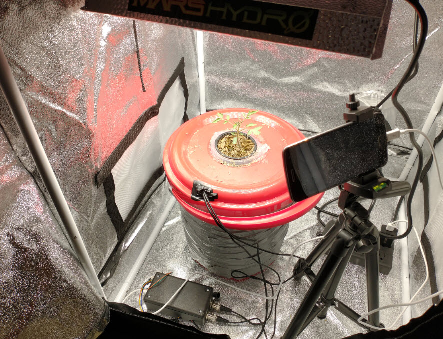
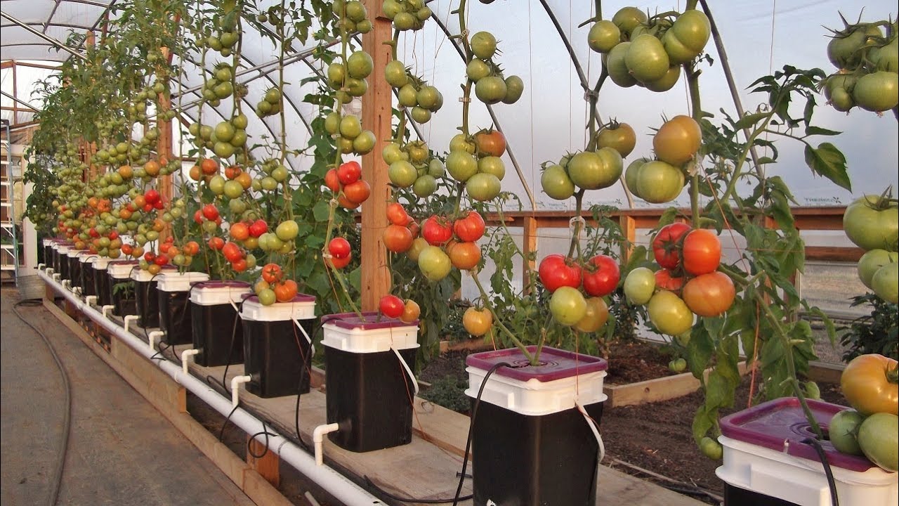
The setup is a 13L bucket wrapped in duct tape – to prevent light from entering the system – with a hole at the top and a net pot containing a tomato plant. The tomato – which I have named Bernard – is an indeterminate cherry tomato that was germinated in the net pot. The net pot contains a medium consisting of 50% rice hulls and 50% river sand. The bucket has been filled with a store-bought generic hydroponic nutrient solution up to the point where it touches the bottom of the net pot. Furthermore, the bucket is placed inside a grow tent and receives 12 hours of light from a Mars Hydro TS 600 Full Spectrum lamp. The light has been initially placed around 10 inches above the plant and will be moved as needed to maintain proper leaf temperature and light coverage of the plant.
The experimental Kratky setup. You can see the project box housing the Arduino and sensor boards at the bottom. Bernard has been growing for 2 weeks and is already showing its second set of true leaves.
The measurements
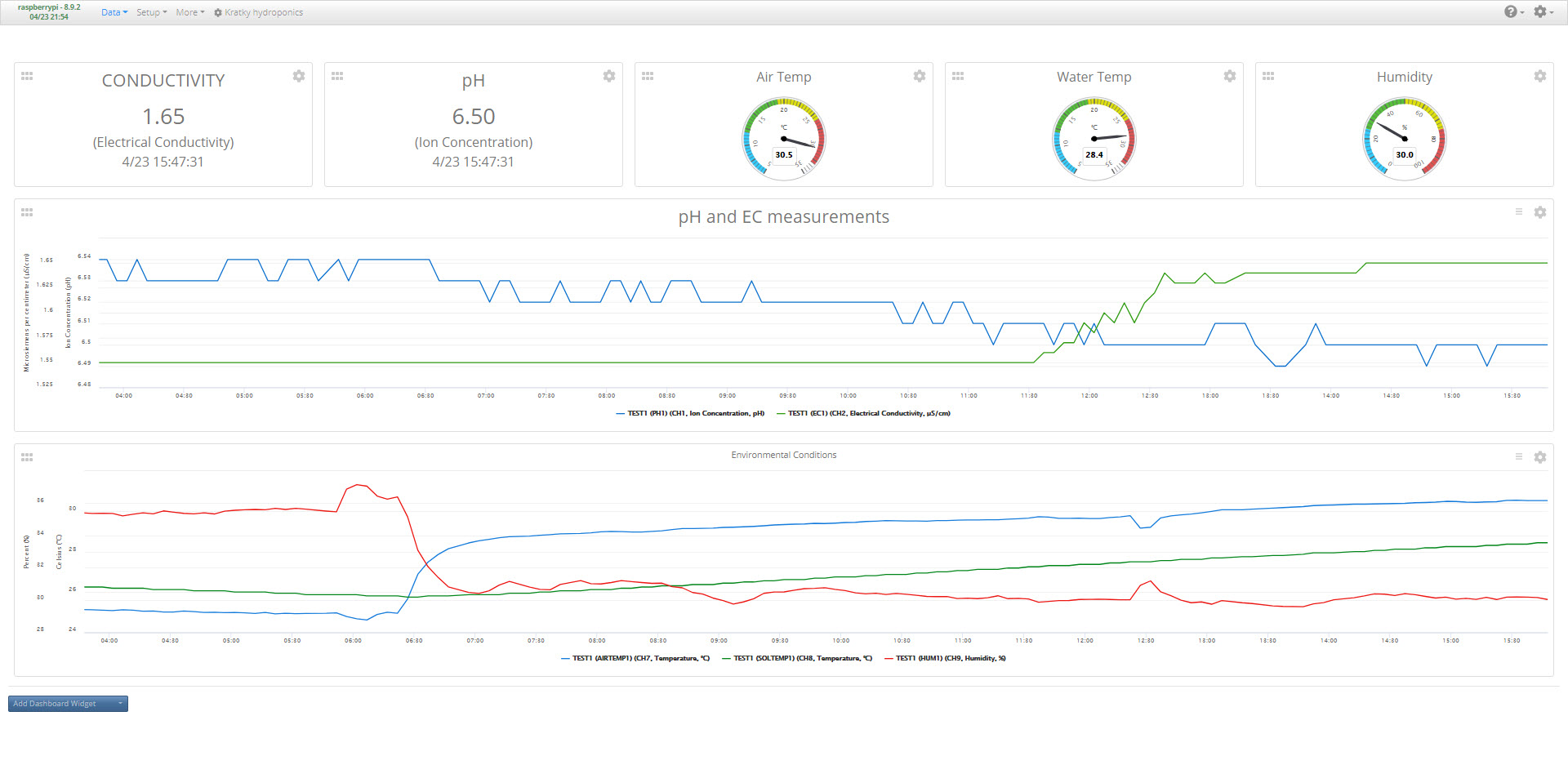
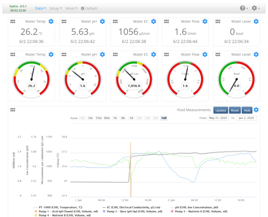
I will be monitoring as many variables as I can within this experiment. To do this I have set up an Arduino MKR Wifi 1010 that uses self-isolated uFire pH and EC probes, a BME280 sensor to monitor air temperature and humidity, and a DS18B20 sensor to monitor the temperature of the solution. I will also be using Horiba probes to track the Nitrate, Potassium, and Calcium concentrations once per day. All the Arduino’s readings are being sent via Wifi to a MyCodo server in a Raspberry Pi, using the MQTT messaging protocol. The data is then recorded into the MyCodo’s database and also displayed in a custom dashboard. The ISE measurements are manually recorded on a spreadsheet.
The dashboard of my MyCodo server, showing the measurements of the system as a function of time. All readings are also recorded in the MyCodo database for future reference and processing.
Furthermore, I am also taking photographs every 15 minutes – when the lights are on – using a smartphone. This will allow me to create a time-lapse showing the growth of the plant from the very early seedling to late fruiting stages.
Conclusion
I have started a new project where I will fully record the complete development process of a large flowering plant in a Kratky setup. We will have information about the EC and pH changes of the solution, as well as information about how different nutrient concentrations (N, K and Ca) change through the life of the plant. With this information, we should be able to figure out how to modify the nutrient solution to grow large flowering plants more successfully, and what interventions might be critical in case fully passive growth is not possible.
I will continue to share updates of this project in both my blog and YouTube channel.
What do you think about this project? Do you think Bernard will make it? Let us know in the comments below!
Arduino hydroponics, how to build a sensor station with an online dashboard
In a previous post about Arduino hydroponics, I talked about some of the simplest projects you could build with Arduinos. We also talked about how you could steadily advance towards more complex projects, if you started with the right boards and shields. In this post, I am going to show you how to build a simple sensor station that measures media moisture and is also connected to a free dashboard platform (flespi). The Arduino will take and display readings from the sensor and transmit them over the internet, where we will be able to monitor them using a custom-made dashboard. This project requires no proto-boards or soldering skills.
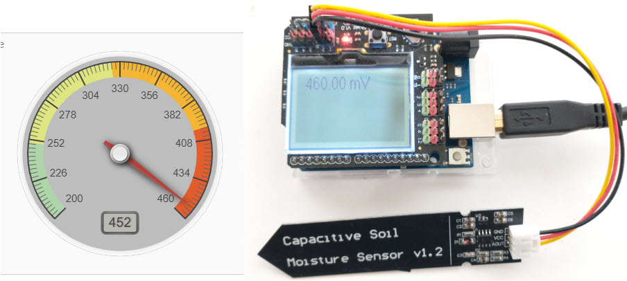
An Arduino Wifi Rev2 connected to a moisture sensor, transmitting readings to an MQTT server hosted by flespi that generates an online dashboard
The idea of this project is to provide you with a simple start to the world of Arduino hydroponics and IoT interfacing. Although the project is quite simple, you can use it as a base to build on. You can add more sensors, improve the display, create more complicated dashboards, etc.
What you will need
For this build, we are going to use an Arduino Wifi Rev2 and an LCD shield from DFRobot. For our sensor, we are going to be using these low-cost capacitive moisture sensors. This sample project uses only one sensor, but you can connect up to five sensors to the LCD shield. Since this project is going to be connected to the internet, it requires access to an internet-connected WiFi network.
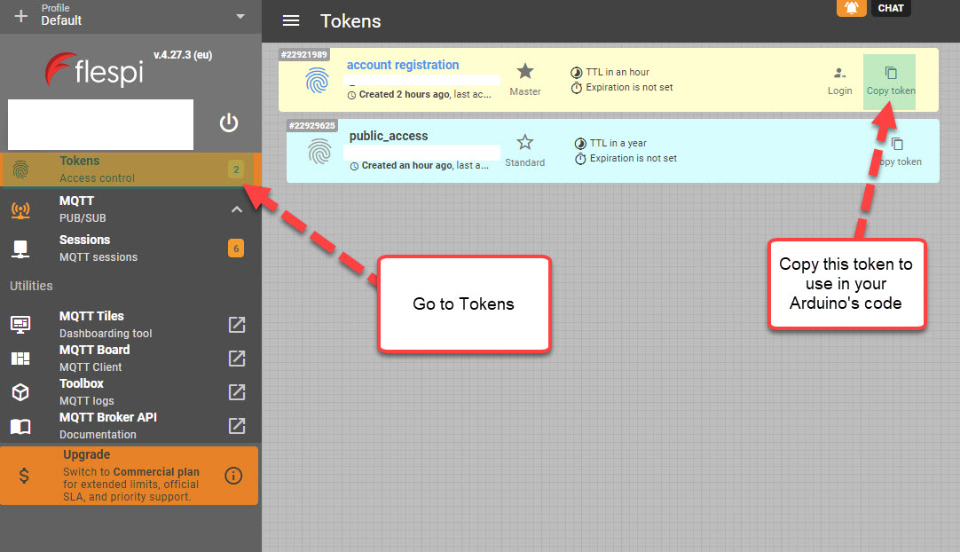
Additionally, you will also need a free flespi account. Go to the flespi page and create an account before you continue with the project. You should select the MQTT option when creating your account since the project uses the MQTT protocol for transmission. After logging into your account, copy the token shown on the “Tokens” page, as you will need it to set up the code.
Copy the token from the “Tokens” menu in flespi
Libraries and code
This project uses the U8g2, ArduinoMQTTClient and WiFiNINA libraries. You should install them before attempting to run the code. The code below is all you need for the project. Make sure you edit the code to input your WiFi SSID, password, and Flespi token, before uploading it to your Arduino. This also assumes you will connect the moisture sensor to the analogue 2 port of your Arduino. You should change the ANALOG_PORT variable to point to the correct port if needed.
#include <Arduino.h>
#include <U8g2lib.h>
#include <WiFiNINA.h>
#include <ArduinoMqttClient.h>
#include <SPI.h>

#define SECRET_SSID "enter your wifi ssid here"
#define SECRET_PASS "enter your password here"
#define FLESPI_TOKEN "enter your flespi token here"
#define ANALOG_PORT  A2

#define MQTT_BROKER    "mqtt.flespi.io"
#define MQTT_PORT      1883

U8G2_ST7565_NHD_C12864_F_4W_SW_SPI u8g2(U8G2_R0, /* clock=*/ 13, /* data=*/ 11, /* cs=*/ 10, /* dc=*/ 9, /* reset=*/ 8);
float capacitance;
WiFiClient wifiClient;
MqttClient mqttClient(wifiClient);

// checks connection to wifi network and flespi MQTT server
void check_connection()
{
  if (!mqttClient.connected()) {
    WiFi.end();
    WiFi.begin(SECRET_SSID, SECRET_PASS);
    delay(10000);
    mqttClient.setUsernamePassword(FLESPI_TOKEN, "");
    if (!mqttClient.connect(MQTT_BROKER, MQTT_PORT)) {
      Serial.print("MQTT connection failed! Error code = ");
      Serial.println(mqttClient.connectError());
      delay(100);
    }
  }
}

void setup() {
  pinMode(LED_BUILTIN, OUTPUT);
  pinMode(4, OUTPUT);
  Serial.begin(9600);
  analogReference(DEFAULT);
  check_connection();
}

void loop() {

  String moisture_string;
  check_connection();

  // read moisture sensor, since this is a wifiRev2 we need to set the reference to VDD
  analogReference(VDD);
  capacitance = analogRead(ANALOG_PORT);

  // form the string we will display on the Arduino LCD screen
  moisture_string = String(capacitance) + " mV";
  Serial.println(moisture_string);

  // send moisture sensor reading to flespi
  mqttClient.beginMessage("MOISTURE1");
  mqttClient.print(capacitance);
  mqttClient.endMessage();

  // the LCD screen only works if I reinitialize it on every loop
  // I also need to reset the analogReference for it to properly work
  analogReference(DEFAULT);
  u8g2.begin();
  u8g2.setFont(u8g2_font_crox3h_tf);
  u8g2.clearBuffer();          // clear the internal memory
  u8g2.drawStr(10,15,moisture_string.c_str());  // write something to the internal memory
  u8g2.sendBuffer();          // transfer internal memory to the display

  delay(5000);

}
Your Arduino should now connect to the internet, take a reading from the moisture sensor, display it on the LCD shield and send it to flespi for recording. Note that the display of the data on the LCD shield is quite rudimentary. This is because I didn’t optimize the font or play too much with the interface. However, this code should provide you with a good template if you want to refine the display.
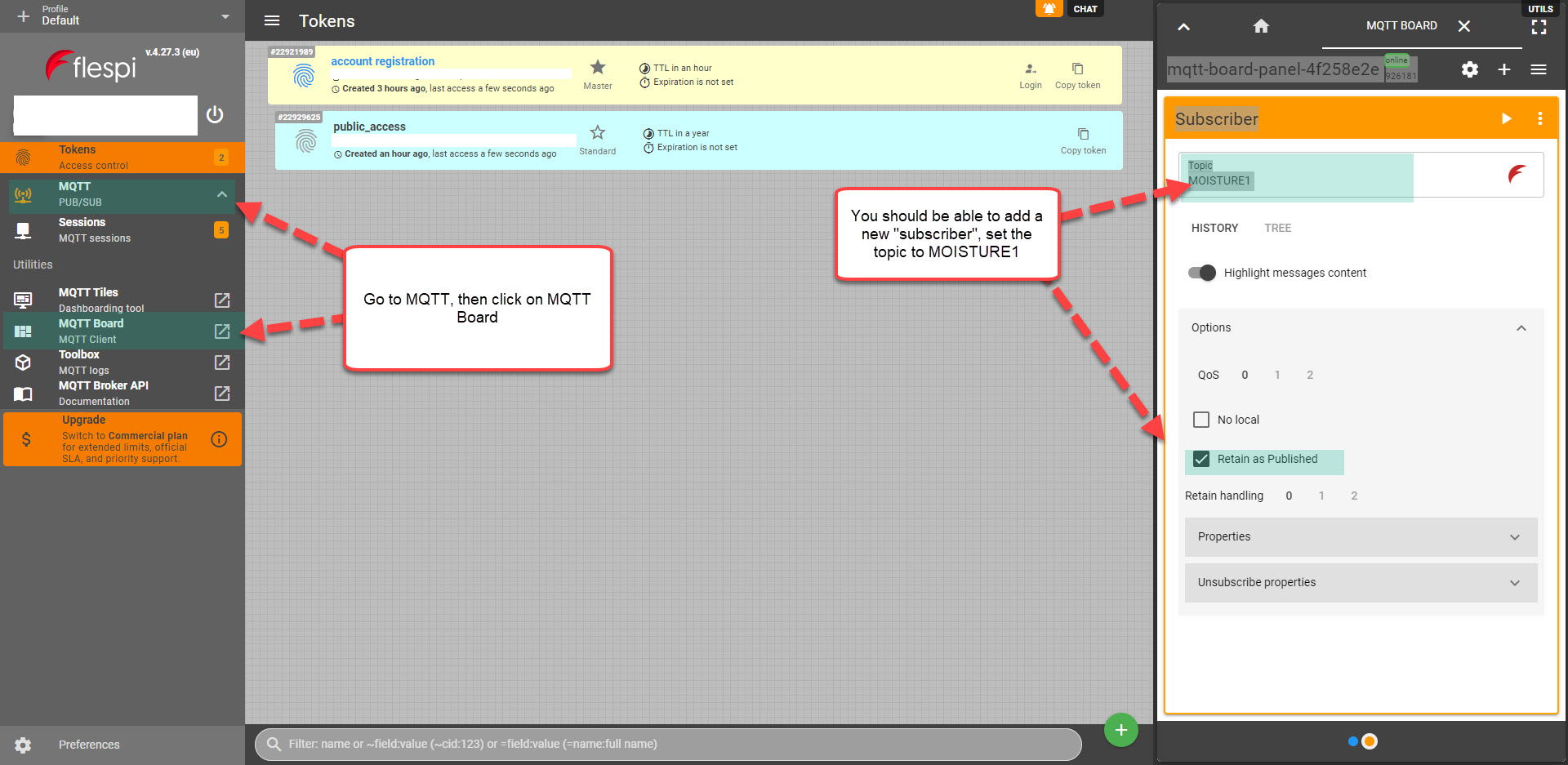
Configure Flespi
The next step is to configure flespi to record and display our readings. First, click the MQTT option to the left and then go into the “MQTT Board” (click the button, no the arrow that opens up a new page). Here, you will be able to add a new subscriber. A “subscriber” is an instance that listens to MQTT messages being published and “MOISTURE1” is the topic that our Arduino will be publishing messages to. If you want to publish data for multiple sensors, you should give each sensor its own topic, then add one flespi subscriber for each sensor.
Go to flespi and create a new “subscriber”, set the topic to MOISTURE1
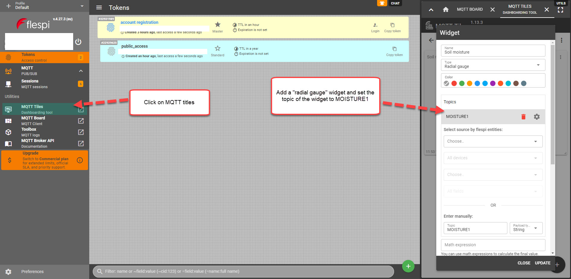
Create the Dashboard
The last step, is to use the “MQTT Titles” menu to create a dashboard. I added a gauge widget to a new dashboard, and then set the topic of it to MOISTURE1, so that its data is updated with our MQTT messages. I set the minimum value to 200; the maximum value to 460; and the low, mid, and high levels to 250, 325, and 400 respectively.
Use the MQTT titles menu to add widgets to a new dashboard
After you finish creating the dashboard, you can then use the “Get link” button, which looks like a link from a chain next to your dashboard’s title. You will need to create an additional token in the “Tokens” menu so that you can use it for the sharing of the dashboard. After you generate the link, it should be publicly available for anyone who is interested. This is the link to the dashboard I created.
Conclusion
You can create a simple and expandable sensor station using an Arduino Wifi Rev2, a capacitive moisture sensor, and an LCD shield. This station can be connected to the internet via Wifi and send its data to flespi, which allows us to create free online dashboards. You can expand on this sensor station by adding more moisture sensors or any other Gravity shield compatible sensors, such as a BME280 sensor for temperature, humidity, and atmospheric pressure readings.
How to choose the best hydroponic bucket system for you
You can use simple buckets to create versatile hydroponic systems. You can create a system to grow a few plants at home or thousands of plants in a commercial facility. However, there are several types of bucket systems to choose from, and making the correct choice is vital to success. In this post, we are going to take a look at the different types of bucket systems. We will examine their pros and cons so that you can better understand them and choose the hydroponic bucket system that best suits your needs.
The Kratky bucket
The simplest system is the Kratky bucket system. In this setup, you have a bucket with one or several holes on the lid. You put plants in net pots with media and then fill the bucket with a nutrient solution so that it is barely touching the bottom of the media. The media initially draws water through capillary action, while the roots reach the nutrient solution. After that, the roots draw nutrients from the water and an air gap is created between the plant and the water as the crop evaporates water. The roots use this air gap to get the oxygen they need for respiration. For this reason, you don’t need any air pumps.
Kratky system using mason jars. I would advice to avoid transparent containers to reduce algae growth.
This completely passive system is easy to build and cheap. You only fill the bucket once with nutrient solution, and you don’t need to check the pH, EC, or other variables through the crop cycle. However, this system requires careful determination of the bucket’s volume, the nutrient solution concentrations, and the crops grown. You can read this post I wrote, for more tips to successfully grow using this bucket system.
However, you cannot easily grow large productive flowering plants in this system. This is because large plants consume too much water and nutrients throughout their life, and will require either a very big volume or complete changing of the nutrient solution at several points. For large flowering plants, it is more convenient to use other types of bucket systems that make solution changes easier. If you would like more information and data regarding the culture of large plants using Kratky hydroponics, please read this post.
The Kratky bucket system is ideal if you need a system with no power consumption, your environmental conditions don’t have extremes, and you want to grow leafy greens or other small plants on a small scale. For larger scales, Kratky systems to grow leafy greens on rafts do exist, although large-scale systems do involve pumps, at least to change solution between crop cycles.
The bucket with and air pump
The Kratky system has zero power consumption, but does require the grower to carefully manage the initial nutrient level and is not very tolerant to strong variations in environmental conditions. For this reason, a more robust method to grow is the bucket with an air stone. This is exactly the same as a Kratky system, except that air is constantly pumped into the nutrient solution and the nutrients are generally maintained at a specific level inside the bucket.
Constantly pumping air into the solution creates several advantages. The first is that air oxygenates the solution, which means the solution’s level is not critical. This is because plant roots have access to oxygen, even if more than the ideal percentage of the root mass is submerged in the solution. The second is that air will help regulate the temperature of the nutrient solution. As air bubbles through and evaporates water, it helps keep the solution cool. Kratky systems can suffer from unwanted temperature spikes if the air temperature gets too hot. This is a common reason for disease and failure in Kratky systems.
A typical air-pump bucket system growing kit
Systems with an air pump are usually easier for people who are just starting. The low cost and low failure rates are the main reason why this is a very popular choice for first-time hydroponic enthusiasts. However, since water evaporates more, there is a need to at least replenish water through the crop cycle. You are also limited to smaller plants unless you’re willing to fully change the nutrient solution several times per crop cycle, which is inconvenient with a bucket system like this. It is also uncommon to see systems like this on a larger scale, as changing and cleaning hundreds of buckets manually and having hundreds of airlines going into buckets is not practical.
Note that air pumps bring substantial amounts of algae into solutions that will thrive if any light can get into your buckets. For hydroponic systems that use air pumps, make sure you use buckets made of black plastic so that no light gets in. White plastic will allow too much light to get in and algae will proliferate.
You can buy several ready-made hydroponic systems of this type. For example this one or this one for multiple small plants.
The Dutch bucket system
A Dutch bucket system is great to grow large plants. In this setup, buckets are connected to drain lines at the bottom. This allows you to pump the nutrient solution into the buckets and allow it to drain several times per day. The constant cycling of solution exposes roots to large amounts of oxygen between irrigation cycles, making this a great setup for highly productive crops.
The Dutch bucket system is therefore an active system, requiring water pumps to keep the plants alive. This dramatically increases the energy consumption needs of the crop and makes the pumps and timers fundamental components of the hydroponic system. An active bucket system like this will usually give the grower 12-24 hours, depending on conditions, to fix critical components in case of failure before plants start to suffer irreversible damage. To prevent damage in commercial operations, drains will usually allow for some amount of water to remain at the bottom of the buckets so that large plants have a buffer to survive more prolonged technical issues.
A commercial Dutch bucket hydroponic system
The need to support the plants without water also means you need to use a lot more media, as the bucket themselves need to be filled with it. Since multiple flood and drain cycles are desirable this also means that the media needs to dry back relatively quickly, reason why media like rice husks, perlite or expanded clay, are used. Media costs of Dutch bucket systems are significantly larger than those of other systems because of this. You can run Dutch bucket systems with netpots as well, but this tends to make the system much less robust to pump failure.
Dutch bucket systems are a good choice if you want to grow highly productive large plants. They offer more robustness when compared with NFT systems – which have more critical points of failure – and the large amount of media provides a good temperature buffer and a great anchoring point for large plants. Several small-scale kits to grow using Dutch buckets also exist (see this one for example). However, they take significantly more space than the alternatives we described before. They require access to power and space for pumps, a large nutrient reservoir, and the supporting infrastructure for the plants. They also require nutrient solution management skills.
Conclusion
Bucket systems are very popular in hydroponics. They can be as simple as a bucket with a hole and a net pot or as complex as Dutch bucket systems with interconnected drain systems and full nutrient solution recirculation.
The easiest system to start with is a hydroponic bucket system with an air pump, as this eliminates the need to gauge the container volume and nutrient level precisely and allows for healthier growth, fewer disease issues, and easier temperature control.
A Kratky system can be great to grow small plants at a low cost with no power, but some experimentation with the nutrient level and concentration is usually required to get a satisfactory crop.
For large plants, the Dutch bucket system is a great choice, if you have the space and power availability. Dutch bucket kits for small-scale growers are also readily available.
Have you ever grown using buckets? Which type of system have you used and why? Let us know in the comments below!
Arduino hydroponics, how to go from simple to complex
Hydroponic systems offer a great opportunity for DIY electronics. In these systems, you can monitor many variables, gather a lot of data, and build automated control systems using this information. However, the more advanced projects can be very overwhelming for people new to Arduinos and the simpler projects can be very limiting and hard to expand on if you don’t make the right decisions from the start. In this post, I’m going to talk about the easiest way to start in Arduino hydroponics, which materials and boards to buy, and how to take this initial setup to a more complex approach with time.
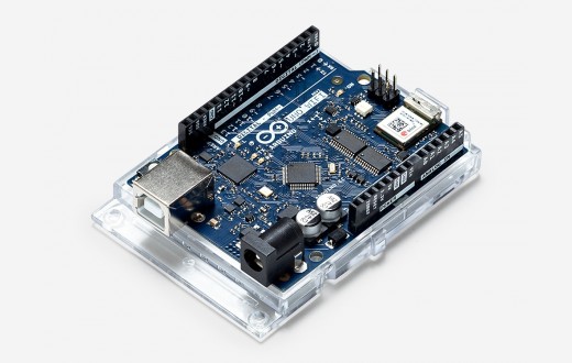
The Arduino Wifi Rev2
Buy the right Arduino
First, buy an Arduino that allows you to build simple projects without compromising your ability to upgrade in the future. My recommendation would be an Arduino Wifi Rev2. These are small boards that are compatible with Arduino Uno shields, with the ability to connect to your network when you’re ready for more complex projects. Shields are boards that can be stacked on top of your Arduino, which allow you to get additional functionality or simplify the usage of the board. The Arduino Wifi Rev2 is a perfect choice, as you can outgrow simpler boards quickly while the more complicated ones are likely to be overkill and limit your potential shield choices.
Avoid soldering and protoboards, go for plug-and-play
For people new to Arduino, it is easier to avoid sensors that require soldering or protoboards and go with plug-and-play approaches. My all-time favorite is the “Gravity” system created by DFrobot, which uses shields that expose quick access connectors that you can use to plug-in sensors. My recommendation is the LCD12864 Shield, which has an LED and allows you to connect both analog and digital sensors. If you buy any “Gravity-compatible” sensor, you will only need to hook up a connector, no soldering or protoboards involved. You also have a graphic interface you can program and buttons you can use to interact with your Arduino and code.
The LCD12864 Gravity shield that exposes easy plug-and-play ports for sensors
Start with a temperature/humidity display station
A good beginner project is to create a monitoring station that displays the readings from sensors on a screen. I’ve written about how to build such a station in a previous blog post. However, since pH and EC sensors can be more complicated, it is easier to start with temperature/humidity sensors only. There are several cheap sensors of this kind, such as the DHT11 and DHT22 sensors, but these have important issues. A better choice for hydroponics is the SHT1x sensor. If you are more advanced, the BME280 sensors are now my low-cost sensor of choice. There are lots of gravity sensors to choose from. You can also monitor CO2, light intensity, solution temperature, EC, pH, and other variables as you become more advanced.
The SHT1x Gravity sensor, this can be easily plugged into the LCD12864 shield shown before
When you go into EC/pH monitoring, make sure you buy sensors that have electrically isolated boards. The ones from DFRobot are not electrically isolated and have important issues when multiple probes are put in the same solution. Most cheap ones on eBay/Amazon, have the same issues. I would recommend the sensors boards from uFire, which have a lower cost, are properly isolated, and are easy to use. The hydroponic kit collection, offers all the sensors and boards you require, in rugged industrial quality configurations, to build a hydroponic monitoring station.
Next step, simple control
The next step in complexity is control. You can use a Gravity relay to switch a light or timer on or off. You can also use a simple dead-band algorithm to attempt to control your temperature and humidity values by using relays to turn humidifiers, dehumidifiers, or AC systems on or off. If you want to control nutrients and pH, this is also where you would get shields to run stepper motors and the peristaltic pumps required to feed solutions into a tank. I’ve used this shield stacked under an LCD12864 for this purpose.
As an example of simple control, imagine your humidity is getting too high, so you install a dehumidifier to keep your humidity from climbing above 80%, you then create a line of code that sets the relay to “on” whenever the humidity gets higher than 80% and shuts it down whenever it drops below 75%. That way your crop’s humidity increases to 80%, the dehumidifier kicks in, and then it shuts down when it reaches 75%. This allows the setup to climb back up for some time, avoiding the continuous triggering of your appliance.
Data Logging
After you’re comfortable with both monitoring setups and simple control, the next step is data logging. Up to this point, none of your setups have done any data logging. By its very nature, an Arduino is not built to log any data, so this will require interactions with computers. My favorite way to do this is to set up a MyCodo server on a Raspberry Pi, then transmit data to it using the MQTT protocol. Since your Arduino Wifi v2 can connect to your Wifi network, you will be able to transmit data to your MyCodo using this configuration.
A sample of the data-logging capabilities of a MyCodo server. Taken from the MyCodo site.
I have previously written posts about MyCodo, as well as how to build a pH/EC wireless sensing station that transmits data to a MyCodo server. This allows me to log data continuously and monitor it without having to go into my hydroponic crop. Since the server is centralized, it also allows you to monitor multiple sensing stations simultaneously. I use my MyCodo server to monitor both my hydroponic crops and Arduino sensing stations that monitor how much food my cats eat.
More complex control
After you have connected your Arduino to a MyCodo server, you have access to much more complicated control, through the Raspberry Pi computer. You can then implement control algorithms in the MyCodo, then communicate with your Arduino, and trigger actions using MQTT messages. This means that you no longer need to code the control logic into your Arduino but you can do all the control in the raspberry Pi and just communicate the decisions made to the Arduino Wifi Rev2.
More complicated algorithms includes the use of proper PID algorithms for the control of humidity, temperature, pH and EC. It also includes the implementation of reinforcement learning algorithms and other advanced control methods that the Raspberry Pi can have the capacity to run.
Conclusion
Arduino in hydroponics does not need to be complex. Your first project can be a simple temperature/humidity monitoring setup and you can evolve to more complicated projects as your understanding and proficiency grow. If you select a powerful and feature-rich Arduino from the start, you can use the same controller through all your different projects. If you select shields that can make your life easier – such as the LCD12864 shield – and use a plug-and-play sensor interface, you can concentrate on building your setup and your code, rather than on soldering, getting connections right, and dealing with messy protoboard setups.
The road from a simple monitoring station to a fully fledged automated hydroponic setup is a long one, but you can walk it in small steps.
Have you used Arduinos in your hydroponic setup? Let us know about your experience in the comments below!
How to get more phosphorus in organic hydroponics
It is difficult to supply plants with readily available phosphorus because of the insolubility of many phosphorus compounds (2). Whenever orthophosphoric acid species are present in a solution, all the heavy metals, calcium, and magnesium form progressively insoluble phosphate salts as the pH increases (3). At high pH, all of the phosphate is expected to be precipitated as long as there are excess cations to form these insoluble salts. In this post, we are going to talk about how this problem exists mainly in organic hydroponics and how we can solve it by efficiently using organic sources of phosphorus.
Seabird guano, one of the few organic, high P, soluble sources for organic hydroponics
Phophorus in traditional hydroponics
In hydroponic systems that are not organic, soluble phosphorus salts are used to provide the phosphorus necessary for plant growth. These salts are all synthetic and are therefore not allowed for use in organic crops. They are mainly mono potassium phosphate (MKP) and mono ammonium phosphate (MAP). At the concentrations generally used in hydroponics – 25-100 ppm of P – at a pH of 5.8-6.2 and in the presence of chelated heavy metals, the phosphorus all remains soluble and there are rarely problems with phosphorus availability that are directly related to the P concentration in solution. However, when trying to move to an organic hydroponic setup where we want to avoid the use of all these synthetic salts, we run into big problems with P availability.
Organic soluble phosphorus fertilizers
The first problem we find is that there are no organic sources that are equivalent to MAP or MKP. However, there are thankfully some highly soluble organic sources that contain significant amounts of P. Some guano sources are particularly high in P, especially Seabird Guano (0-11-0), while some vegetable sources like corn steep liquor (CSL) (7-8-6) can also have high phosphorus (1, 9).
However, these sources do not only contribute phosphorus but will also contribute a variety of different substances that need to be taken into account when considering them for use. In the case of CSL, very high lactate and organic nitrogen levels imply that you will need to prepare an appropriate compost tea to use this in a nutrient solution. I wrote a blog post about a paper that describes how to make such a preparation.
In the case of seabird guano, a lot of calcium is also provided (20%) so we also need to take this into account in our formulations. Using 3g/gal of seabird guano will provide you with a solution that contains 38ppm of P and 158ppm of Ca, although not in exactly readily available form – as MKP would provide – it will become available much easier than insoluble phosphate amendments. Seabird guano applications should be enough to completely cover both the P and Ca requirements of most flowering plants. The seabird guano also includes a lot of microbial activity, which will reduce the oxygenation of the media when it is applied, reason why you need to be careful with the aeration properties of your media (as I mentioned in this post).
These organic sources of P might also contain significant amounts of heavy metals. Seabird guano can be notable for having significant levels of cadmium (4, 5) so make sure you have a heavy metal test of the soluble P source you intend to use to ensure you’re not adding significant amounts of heavy metals to your crops.
Insoluble organic phosphorus amendments
Besides these soluble organic phosphorus sources, we also have the possibility to use mineral amendments that can be directly incorporated into the media from the start. These sources offer us some additional advantages relative to the pH and nutrient stability through time, which are not offered by using the soluble solutions. The most common amendments available in this area are rock phosphates and bone meal. Not all rock phosphates and bone meal sources are created the same though, rock phosphates mined across the world can differ in their carbonate content, which can greatly affect their solubility. These amendments are generally used at around 60-120mL per gallon of soil.
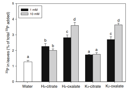
P uptake for different concentrations of citrate or oxalate.
Plants, however, will respond to low P in their root zone by releasing organic anions that can chelate metals and slowly dissolve these phosphates (6). Tests by adding organic acids directly do show that not all acids are the same and some are much more effective than others. In this article (7), the authors showed that oxalic acid was more effective than citric acid in making P available from a rock phosphate source. Malic acid, a very important organic acid for plants (8), can also be used for this purpose and is preferable to oxalic acid. This is because oxalic acid is not only toxic to humans but can also strongly precipitate metals like iron, which are also needed by plants.
From the literature, we can conclude that adding these acids ourselves in concentrations of around 1mM, can be a good way to help solubilize P contained in these rock phosphate amendments. Watering with a solution of citric or malic acid at 150mg/L (567mg/gal) can help free these rock phosphate amendments and contribute to plant absorption of both the phosphorus and the calcium that is bound with it. Alternatively, we can also use fulvic acid at 40mg/L to achieve a similar effect (10).
Conclusion
While there are no easy replacements for phosphorus in organic hydroponics, there are some satisfactory solutions. Soluble phosphorous sources like CSL and seabird guano can be used to provide large amounts of soluble P when required, while solid amendments like rock phosphate and bone meal can provide a sustained release of these nutrients with time, also increasing the pH stability of the media. While using only soluble sources can be the easiest initial transition from a purely hydroponic crop, it will also be harder to manage due to the effects on media pH that such applications might have. A combination of both approaches – soluble applications and amendments – can often be the most successful when implementing an organic hydroponic approach.
Organic nitrogen in hydroponics, the proven way
Nitrogen is a critical nutrient for plants. In hydroponics, we can choose to provide it in three ways, as nitrate, as ammonium or as organic nitrogen. This last choice is the most complex one. It contains all possible nitrogen-containing organic molecules produced by organisms, such as proteins and nucleic acids. Since nitrate and ammonium are simple molecules, we know how plants react to them, but given that organic nitrogen can be more complicated, its interactions and effects on plants can be substantially harder to understand. In this post, we will take an evidence-based look at organic nitrogen, how it interacts in a hydroponic crop and how there is a proven way to use organic nitrogen to obtain great results in our hydroponic setups.
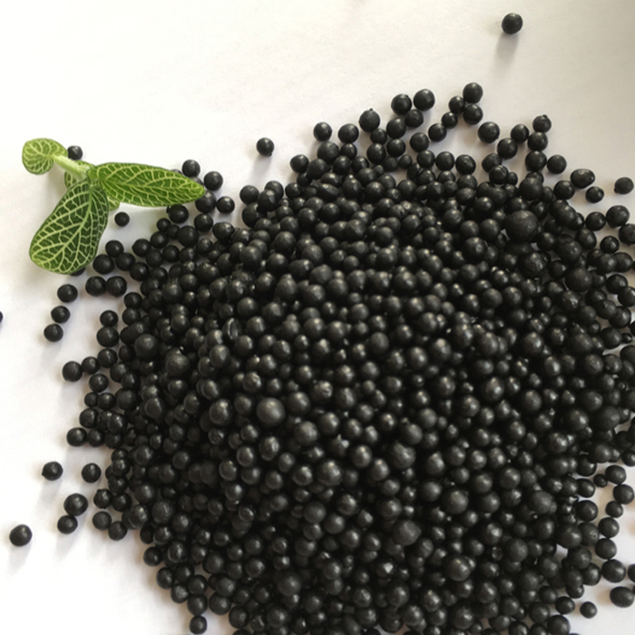
An organic nitrogen source, product of corn fermentation, rich in protein and humic acids
Nitrogen uptake by plants
The main issue with organic nitrogen is its complexity. Plants will mainly uptake nitrogen as nitrate (NO3–) and will also readily uptake nitrogen as ammonium (NH4+) to supplement some of their nitrogen intake. However, organic nitrogen is made up of larger, more complex molecules, reason why its uptake is more complicated. Various studies have looked into whether plants can actually uptake organic nitrogen directly at all (1, 2). They have found that while some uptake is possible, it is unlikely to be the main contributor to a plant’s nitrogen uptake. While plants might be able to uptake this organic nitrogen to some extent, especially if it is comprised of smaller molecules (3, 6), it is unlikely that this nitrogen will be able to replace the main absorption pathway for nitrogen in plants, which is inorganic nitrate.
Effects of organic nitrogen in hydroponics
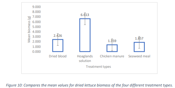
Many researchers have tried to figure out what the effect of organic nitrogen is in hydroponics. This study (4), looked at the effect of various organic nitrogen sources in the cultivation of lettuce. The study tried to measure how these fertilizers compared against a complete Hoagland solution. The results show that the organic nitrogen sources were unable to successfully compete with the standard mineral nutrition. The best result was obtained with blood meal, with less than half of the yield obtained from the Hoagland solution. It is clear that this study is not fair, as using organic nitrogen sources as the sole source of nutrition means more deficiencies than simply nitrogen might be present, but it does highlight some of the challenges of using organic nitrogen in hydroponics.
Another study (5), performed a more direct comparison of various different nitrogen sources, changing only the nitrogen source between nitrate, ammonium, and organic nitrogen in the cultivation of tomatoes. Organic nitrogen performed the worst across most measurements in the study. This showed that organic nitrogen is, by itself, not a suitable form of nitrogen for plant absorption and is unable to replace the nutrition provided by a synthetic inorganic nitrate source. This is especially the case when the organic nitrogen comes from more complex sources.
As we’ve seen, the main problem with organic nitrogen is that plants cannot uptake it efficiently. However, the nitrogen cycle provides us with mechanisms to convert organic nitrogen into mineral nitrate which plants can readily metabolize. The best way to achieve this is to prepare compost teas using the organic nitrogen source to create a nutrient solution that is better suited for plants. The use of nitrifying organisms provides the best path to do this. These organisms are present in a variety of potting soils and composts, but can also be bought and used directly.
This study (7) showed how using goat manure coupled with nitrifying bacteria was a viable path to generate a nutrient solution suitable for plant growth. Another study (8), also using manure, confirms that viable nutrient solutions can be created and used to grow crops successfully when compared to hydroponic controls. Manure, as an animal waste product, contains a lot of the macro and micronutrients necessary for plant growth, providing an ideal feedstock for the creation of a full replacement for a nutrient solution.
Another interesting study (9) uses vegetable sources in order to study the creation of such solutions. I recently used this study to create a detailed post about how to create a nitrate-rich compost tea for use in hydroponics starting from corn steep liquor and bark compost as inputs.
In conclusion
Organic nitrogen sources, by themselves, are not suitable as the main source of nitrogen for plant growth. This is especially true of very complex nitrogen sources, such as those contained in blood meal, corn steep liquor and fish emulsions. However, we can take advantage of nitrifying bacteria and use these inputs to create nitrate-rich solutions that can be used to effectively grow plants.This is a proven solution that has been tried and tested in multiple studies and in nature for hundreds of thousands of years. Instead of attempting to use organic nitrogen sources either directly in the hydroponic solution or as media amendments, create compost teas with them that contain readily available mineral nitrate instead.
Do you use organic nitrogen in hydroponics? What is your experience?
Aquaponics vs hydroponics, which is best and why?
In hydroponic culture, plants are grown with the help of a nutrient solution that contains all the substances required for plant growth. In these systems, the nutrient solution is prepared using externally sourced chemicals, which can be of a synthetic or natural origin. On the other hand, in aquaponics, a plant growing system is coupled with an aquaculture system – a system that raises fish – so that the plants feed on the waste coming from the fish. In theory, aquaponics offers the benefits of a simplified, closed system with an additional upside – the ability to produce fish – while a hydroponic system requires a lot of additional and more complicated inputs. Through this post, we will use the current peer-reviewed literature to take a deep look into aquaponics vs hydroponics, what are the advantages and disadvantages and why one might be better than the other. A lot of the information below has been taken from this 2019 review on aquaponics (9).
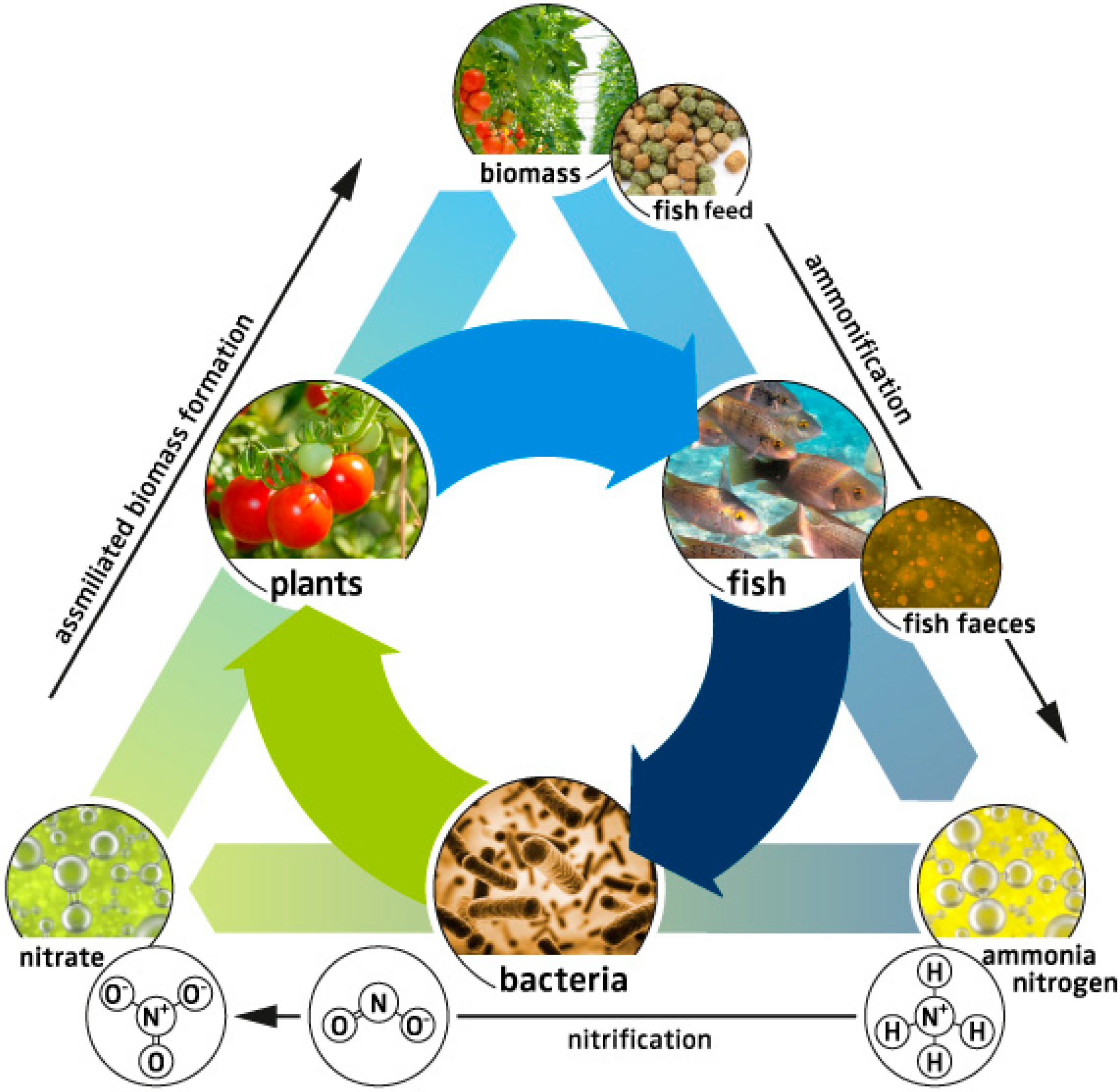
Basic process diagram of an aquaponic setup (from here)
Complexity
An aquaponic system might seem simpler than a hydroponic system. After all, it is all about feeding fish regular fish food and then feeding the waste products to plants. However, it is actually not that simple, since there are substantial differences between the waste products of fish and the nutritional needs of plants. One of the most critical ones is nitrogen.
This element is excreted by fish in its ammoniacal form but plants require nitrogen in its nitrate form. This means that you need to have a biofilter system containing bacteria that can turn one into the other. Furthermore, the chemical conditions ideal for nitrification are basic, while plants prefer solutions that are slightly acidic. This mismatch in the optimal conditions of one system compared to the other makes the management of an aquaponic system substantially more complicated than the management of a traditional hydroponic system (1).
Furthermore, plant macronutrients like Potassium and Calcium and micronutrients like Iron are often present at low levels in aquaponic solutions. Plants that have higher demands for these elements, such as large flowering plants or some herbs, might have important deficiencies and issues when grown in an aquaponic system (2, 3). This means that supplementation is often required in order to achieve success with these crops. Achieving ideal supplementation rates often requires chemical analysis in order to properly gauge the amounts of these elements that are required.
Additionally, aquaponic systems require additional area for fish and a lot of additional labor to manage the fish, the biofilters, and other sections of the facility that would not exist under a purely hydroponic paradigm. This article (16), better describes some of the economic and practical tradeoffs in terms of complexity when going from a hydroponic to an aquaponic facility.
Yield and quality
Given the above, it could be easy to think that yields and quality of products coming from aquaponics would be worse. However, the evidence points to the contrary. Multiple studies looking at aquaponics vs hydroponics quality and yields have shown that aquaponics products can be equivalent or often superior to those produced in hydroponic environments (4, 5, 6, 7, 8). A variety of biological and chemical factors present in the aquaponic solution could offer bio-stimulating effects that are not found in traditional hydroponic solutions. For a detailed meta-analysis gathering data from a lot of different articles on aquaponics vs hydroponics see here (14).
The best results are often found with decoupled aquaponic systems. In these systems, the aquaponic system is treated as separate aquaculture and hydroponic systems. The nutrient solution is stored in a tank that is used by the hydroponic facility as its main feedstock to make nutrient solution. Its chemistry is then adjusted before it is fed to the hydroponic system.
An aquaponic setup growing leafy greens
Growing Systems
Traditionally, Nutrient Film Technique (NFT) systems have been preferred in commercial hydroponic culture due to their high yield and effectiveness. However, aquaponic systems do better with setups that can handle large levels of particulates, due to their presence in the aquaponic nutrient solution. For this reason, deep water culture (DWC) is the preferred method for growing in commercial hydroponic systems. This is also because dark leafy vegetables are the most commonly grown products in aquaponic setups and DWC setups are particularly well suited to grow this type of plants.
Sustainability
Aquaponic systems are, on average, more sustainable than hydroponic systems in terms of fertilizer usage. When comparing Nitrogen and Phosphorus usage between a hydroponic and an aquaponic crop, it seems to be clear that aquaponic crops are much more efficient (12). An aquaponic crop can offer the same quality and yield with drastically lower fertilizer use and carbon dioxide emissions due to these facts (13).
The aquaponic closed system diagram, taken from here
The economics
Due to the poor nutritional characteristics of the aquaponic solutions for flowering plants, most aquaponic growers have resorted to the growing of leafy greens. A 2017 study (10) showed that profits from growing basil were more than double of those attained by growing Okra, due to the fact that basil could be grown with little additional supplementation while Okra required significant modification of the aquaponic solution to fit the plants’ needs.
Due to the fact that large flowering plants require large amounts of mineral supplementation in order to be grown successfully in aquaponics, they are seldom grown in aquaponics setups. Since leafy greens eliminate the need for such supplementation, can be grown faster, and suffer from substantially less pest pressure, it is a no-brainer in most cases to grow leafy greens instead of a crop like tomatoes or peppers. However, high-value crops like cannabis might be attractive for aquaponics setups (10, 11).
Aquaponics often require economies of scale to become viable. The smallest scale aquaponic setups, like those proposed by FAO models, can offer food production capabilities to small groups of people, but suffer from a lack of economic viability when the cost of labor is taken into account (12). It is, therefore, the case that, to be as profitable as hydroponics, aquaponic facilities need to be implemented at a relatively large scale from the start, which limits their viability when compared with hydroponic setups that can offer profitability at lower scales. As a matter of fact, this 2015 study (15) showed that most aquaponic farms were implemented at relatively small scales and had therefore low profitability values.
Nonetheless, aquaponics does offer a much more sustainable way to produce food relative to conventional hydroponic facilities and does offer economic advantages, especially in regions where low water and fertilizer usage are a priority (14).
Which one is best then?
It depends on what your priorities are. If you want to build a setup with few uncertainties that can deliver the most profit at the smallest scale, then hydroponics is the way to go. Aquaponic setups have additional complexities, uncertainties, needs of scale, and limitations that hydroponic crops do not have. Building a hydroponic commercial setup is a tried-and-tested process. Hydroponics offers predictable yields and quality for a wide variety of plant products. There is also a wide industry of people who can help you achieve this, often with turn-key solutions for particular plant species and climates.
On the other hand, if you want to build a setup that is highly sustainable, has as little impact as possible on the environment, has very low fertilizer and water use and can deliver the same or better quality as a hydroponic setup, then aquaponics is the road for you. Aquaponics has significantly lower impact – as it reduces the impact of both plant growing and fish raising – and can deliver adequate economic returns if the correct fish and plant species are chosen.
In the end, it is a matter of choosing which things are most important for you and most adequate for the circumstances you will be growing in. Sometimes, limited fertilizer and water availability, coupled with higher demand for fish, might actually make an aquaponic setup the optimal economic choice versus a traditional hydroponic setup. However, most of the time a purely economic analysis would give the edge to a hydroponic facility.
If you are considering building an aquaponic system, a decoupled system that produces Tilapia and a deep water culture system producing dark leafy greens seems to be the most popular choice among commercial facilities.
Which do you think is better, aquaponics or hydroponics?
The ultimate EC to ppm chart and calculator
Electrical conductivity (EC) meters in hydroponics will generally give you different types of readings. All of these readings are conversions of the same measurement – the electrical conductivity of the solution – but growers will often only record one of them. The tools presented in this page will help you convert your old readings from one of these values to the other, so that you can compare with reference sources or with readings from a new meter. In this page you can figure out the scale of your meter, convert from ppm to EC and from EC to ppm.
The TDS reading of different meters will be done on different scales, so it is important to know the scale of your meter in order to perform these conversions. These scales are just different reference standards depending on whether your meter is comparing the conductivity of your solution to that of an NaCl, KCl or tap water standard. To learn more about how TDS scales work I would suggest you watch my youtube video on the subject. To compare the readings from different meters, always compare the EC (mS/cm) reading, do not compare ppm readings unless you are sure they are in the same scale.
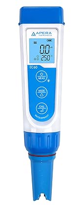
My go-to EC meter recommendation is the Apera EC60
To figure out the scale of the meter, measure the EC (mS/cm) and TDS (ppm) of the exact same solution with your meter. After this, input the values in the first calculator below. You can then use this scale value to convert between EC and ppm using the other two calculators below. If you already know the scale of your meter you can use the other two calculators and skip the first step. The meter scale will usually be 500, 600 or 700.
Figure out the Scale of the Meter
TDS (ppm) reading:
EC (mS/cm) reading:
Meter scale:
Convert ppm to EC
TDS (ppm) reading:
Meter scale:
EC in mS/cm:
Convert EC to ppm
EC reading mS/cm:
Meter scale:
TDS (ppm) reading:
Create a table for reference
Meter scale:
If you would like to learn more about EC readings in hydroponics I would suggest reading the following posts on my blog:
Ebb and flow or “flood and drain” systems, are some of the most popular systems built in hydroponics. These are low cost, can host a large number of plants, and can generate good results, reason why they are a preferred choice for both new and experienced hydroponic growers. However, there are a substantial number of issues that can come up in these systems, both due to the different ways they can be built and because of failures in their management. In this post, I am going to give you some tips on the construction and management of ebb and flow systems so that you can minimize the chances of failure when building your own hydroponic setup of this kind. For some basics of how an ebb and flow system is set up, I advise you to watch this video.
Ensure full drainage
A common mistake when building a flood and drain system is to have incomplete drainage of the nutrient solution. Make sure you have a setup that allows for complete drainage of the solution as soon as a certain level is reached, and always stop pumps as soon as the return of the solution starts. It is quite important to also ensure that as little solution as possible remains at the bottom of your flood and drain trays or buckets, as plants sitting in puddles of water can be a recipe for disease and a very good environment for pests to develop. A very simple system I built in 2010 had the problem of never being able to efficiently drain, which caused substantial issues with the plants as root oxygenation was never as good as it should have been.
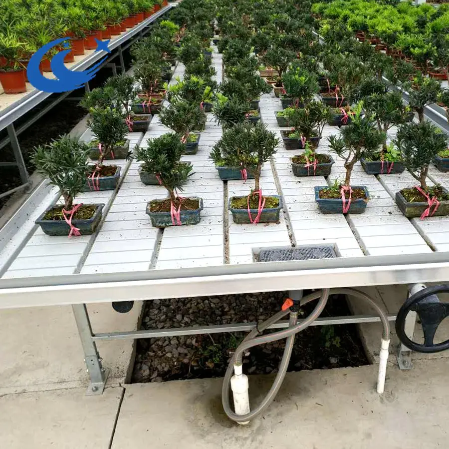
Typical flood and drain table with plants in media on top of the table.
Fast cycle speed
Ideally, you would want the flood and drain cycle of an ebb and flow system to be as fast as possible. Also, the cycles should not take more than 15 minutes, from starting to flood the growing table to completely draining the system. For this, you need to have an adequately sized pump for the volume of your table that needs to be filled (total volume minus volume taken up by plants and media). If you want to use a smaller pump, you can always add some rocks to the table in order to take up volume and ensure you require to add less volume to fully flood the reservoir. Time your cycles and make sure these are as short as possible, adequately saturate the media and completely drain, as mentioned above.
The right media
A common reason why flood and drain systems are less productive is because of a suboptimal choice of media. Ebb and flow systems periodically flood the media with nutrient solution, completely saturating it with water, so media that retains too much moisture will require infrequent cycles and will be harder to time. Media like peat moss and coco are often inadequate for ebb and flow systems due to this fact, as over-saturation of the media will lead to periods of low oxygen availability for the plants. Media that drain fast generally do much better, choices such as rockwool or perlite can give much better results when compared with media that have much higher moisture retention. Since this is a recirculating setup, perlite and rockwool also have the advantage of being more chemically inert. I however do not like media that drain too fast, such as clay pellets, as these can require too frequent cycling.
Another typical ebb and flow table setup
Time irrigations with water content sensors
Your flood and drain system requires good timing of irrigation cycles in order to have optimal results. If you irrigate based on a timer, you will over irrigate your plants when they are small and will under irrigate them when they are big. Overwatering can be a big problem in these systems and it can be completely solved by both choosing the right media – as mentioned above – and using capacitive water content sensors for the timing of your irrigations. If you’re interested in doing this, check out this post I wrote about how to create and calibrate your own simple setup for using a capacitive water content sensor using an Arduino. This will allow you to flood your table only when it is needed and not risk over watering just because of a timed event happening.
Oversize the reservoir
The nutrient reservoir contains all the nutrition that is used by the plants, this means the bigger this is relative to the number of plants you have, the lower the impact of the plants per irrigation event will be. Having a reservoir that has around 5-10 gallons per plant – if you’re growing large flowering plants – or 1-3 gallon per plant, for leafy greens, will give you enough of a concentration buffer so that problems that develop do so slowly and are easier to fix. A large reservoir can fight the effects of plants more effectively and make everything easier to control.
Add inline UV sterilization
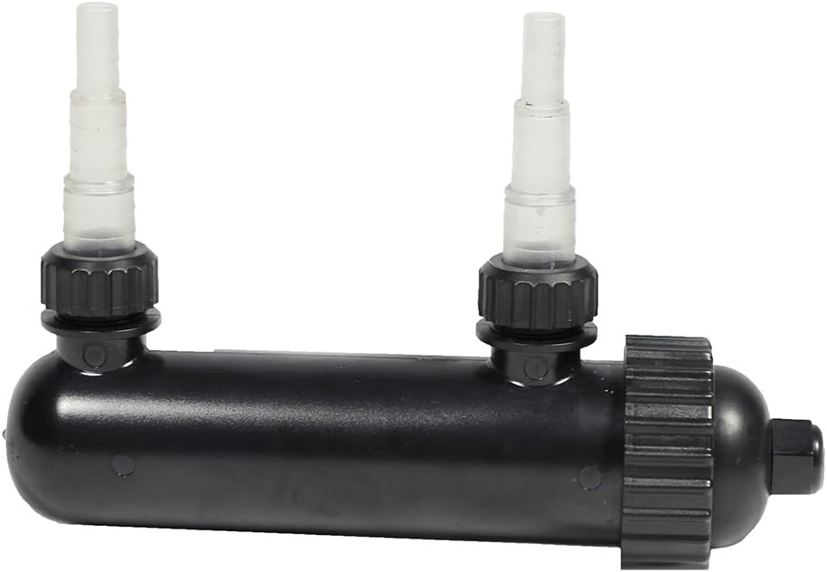
Disease propagation is one of the biggest problems of this type of system. Since recirculation continuously redistributes any fungal or bacterial spores among all the plants, it is important to ensure you have a defense against this problem. A UV filter can help you maintain your reservoir clean. You can run the solution through the inline UV filter on every irrigation event, ensuring that all the solution that reaches the plants will be as clean as possible. Make sure you use a UV filter that is rated for the gallons per hour (GPH) requirements of your particular flood and drain system. Also read my post about getting read of algae, to learn more about what you can do to reduce the presence of algae in a system like this.
Typical UV in-line filter used to sterilize a nutrient solution in a hydroponic setup. These are sold in aquarium shops as well.
Run at constant nutrient EC, not reservoir volume
One of the easiest ways to manage a recirculating system, especially with an oversized reservoir, is to keep it at constant EC instead of constant volume. This means you will only top it off with water in order to bring the EC back to its starting value, but you will never add nutrients to the reservoir. This will cause your total volume to drop with time as you will be adding less volume each time to get back to the original EC. When the volume drops to the point where you have less than 50% of the original volume, completely replace your reservoir with new nutrients. This gives you a better idea of how “used up” your solution really is and how close to bad imbalances in the nutrient solution you might be. A large flowering plant will normally uptake 1-2L/day, meaning that with a reservoir sized at around 5 gallons per plant, it will take you around 2-3 weeks to replace the water.
Note that more efficient and complicated ways to manage a nutrient reservoir exist, but the above is a very safe way to do so without the possibility of toxic over accumulations of nutrients from attempts to run at constant volume by attempting to add nutrients at a reduced strength to compensate for plant uptake. Topping off with nutrients without regard for the changes in the nutrient solution chemistry can often lead to bad problems. The above approach is simple and gives good results without toxicity problems.
Change your pH according to the return pH values
Instead of watering at the normal 5.8-6.2 range, check the pH of the return on a drain cycle to figure out where you should feed. Since a flood and drain system is not a constantly recirculating system, the solution conditions do not necessarily match the root zone conditions and trying to keep the solution at 5.8-6.2 might actually lead to more basic or acidic conditions than desired in the root zone. Instead, check for the return pH to be 5.8-6.2, if it is not, then you need to adjust your reservoir so that it waters at a higher or lower pH (always staying in the 5-7 range) in order to compensate for how the root zone pH might be drifting. This can take some practice, but you can get significantly better results if you base your pH value on what the return pH of your solution is, rather than by attempting to set the ideal pH at the reservoir. You will often see that you will be feeding at a consistently lower pH 5.5-5.6, in order to accommodate nutrient absorption.
Finally
The above are some simple, yet I believe critical things to consider if you want to succeed with an ebb and flow system. The above should make it much easier to successfully run a setup of this kind and grow healthy and very productive plants. Let me know what you think in the comments below!
The value of Fulvic Acid in hydroponics
Fulvic and humic acids have been studied for decades and used extensively in the soil and hydroponic growing industries. I previously talked about the use of humic acid in hydroponics and the way in which it can improve crop results. In that post, we talked about how humic acids can improve nutrient chelation and how this can lead to improvements in yields depending on the origin and properties of the humic substances used. In this post, we are going to take a look specifically at fulvic acid substances, which are a smaller family that has potentially more valuable uses in the hydroponic space. We will start by discussing what differentiates fulvic and humic acids and what the current peer-reviewed evidence around fulvic acids tells us.
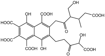
This is a model of the general type of molecule that makes up fulvic acid. Note that fulvic acid is not a pure substance, but a mixture of many substances with similar chemical properties.
Fulvic acids are not chemically pure substances, but a group of chemicals that result from the decomposition of organic matter. This process generates both humic and fulvic acids. However, fulvic acids are different from humic acids in mainly two ways. The first is that fulvic acids are soluble at both acid and alkaline pH values, and the second, is that fulvic acids generally have much lower molecular weights. Fulvic acids are therefore more soluble and are more easily accessible to plants compared to humic acids, which have much larger molecular weights. But why should we use them in hydroponics and exactly how?
Sadly, not many publications have tackled the use of fulvic acid in crops specifically. One of the few examples of reviews that touch on the matter is this paper, which covers most of the literature around fulvic acids before 2014. I also did a literature review myself, trying to find articles in which the fulvic acid source, application type and rate, and the results against a control without fulvic acid were clearly explained. The table below shows you the results of my search, I was able to find 10 papers overall, with a mix of root and foliar applications of fulvic acid, with a range of application rates and plant species. Almost all of these papers found positive results from the use of fulvic acid, except two papers that found either no effect or mixed results from their use.
The range of application depends substantially on the application type. Most papers that tackled foliar applications chose application rates in the 1-3g/L range, while papers that tackled root applications generally stayed in the 25-150ppm range. This is normal since foliars are generally much more concentrated than root applications. Both types of applications have different effects. Root applications are going to exercise an additional strong nutrient chelating role, while foliar applications are more likely to exert a hormonal role. A study around genetically modified tomato plants showed that plants engineered to be insensitive to IAA were also unable to respond to fulvic acid, hinting at the fact that fulvic acid has an auxin-like effect in plants.
Literature search of fulvic acid related publications. The websites where you can read the articles are linked in the “Ref” column.
The effects seem to be quite positive overall, with increases in yield, quality, and flower numbers across the board. The studies above that investigated nutrient transport also showed substantial benefits when root applications of fulvic acid were used. Plants grown in a Hoagland solution showed better nutrient transport when fulvic acid substances were used in the nutrient solution. This is possibly both due to their ability to chelate micronutrients and their ability to provide an additional pH buffer at the region of interest in hydroponics (5.5-6.5). This study, shows how fulvic acid substances can have pKa values in this precise region, although their still relatively large molar mass implies that they will contribute marginally to buffering capacity, especially if used only in <100 ppm concentrations.
Fulvic acids also seem to be synergistic with several other biostimulants in the studies showed above. When tests were done with humic acids or other biostimulants, the effect of the combination is usually better than the effect of either part on its own. This means the fulvic acid might not only be a good addition on its own, but it might also contribute significantly to enhance the effect of other biostimulants used.
It is however important to note that fulvic acids do have negative effects when used in excess, reason why their application rates need to be carefully controlled. Using too much can lead to drops in yields and quality along with slower growth. If you want to start using them, it is, therefore, wise to start at the lower range of the application rates shown above and climb up as you gauge the effects. It is also important to note that – as humic acids – different sources of fulvic acid might have different effects, as the actual molecules that make up the substance will change.
A big advantage of the use of fulvic acids in hydroponics is also that their solubility is quite high, so the risk of clogging or damaging equipment is low. This is a significant advantage over humic acids, which have lower solubility and can cause problems because of this in hydroponics culture, especially if there are drops in the pH. In hydroponics, fulvic acids can also lead to additional solution stability, especially in recirculating systems, where the destruction of heavy metal chelates as a function of time can become a bigger risk.
All in all, fulvic acids represent a relatively cheap addition to a hydroponic regime that has limited risk and a lot of potential upsides. Literature research shows us that low rate applications, if anything, might just have no effect, so the risk of damage to a hydroponic crop by trying fulvic acid applications is low. The synergistic effects shown by fulvic acid are also interesting since this means that they might make other additives you are currently using even more potent. When looking for fulvic acids, make sure you check for high solubility, solubility in low and high pH, and a source that matches the sources used in the literature results you’re interested in reproducing.