Making the most out of your hydroponic setup’s logged sensor and control data
If you have a hydroponic crop with a data logging and automated control solution, you probably have a lot of sensor and control data recorded that could be useful to take your crop’s results to the next level. In this post, I am going to talk about some things that you could be doing with these stored data. You will see how the usage of this data opens up many possibilities and that even implementing the most basic of these suggestions could lead to important improvements in your understanding of your crop and its results.
The lowest hanging fruit to take advantage of logged data is to be able to download the data and put it into a database structure that you can properly query and search. Most data logging solutions record the data in either very simple structures, like csv files, or non-relational databases – like MongoDB – which are rather limited and do not allow for the degree of versatility that a true relational database engine offers. Having the data in a properly built database will allow you to start using it in a creative way. For example, with the data in a proper database, it becomes possible to create a custom data visualization that can help you understand what’s going on inside your growing environment.
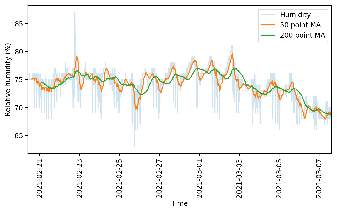
The images in this post show you some examples of this. The first one shows a simple example where a rather noisy humidity sensor is smoothed out using different moving averages, these averages can then be used to implement more effective control algorithms. The second image shows a detailed map of the temperature and humidity values experienced in a room, colored by the hour of the day. We can use this plot to easily locate where problematic times and VPD conditions might be, just by looking at when extreme readings happen. This behavior would be harder to observe and diagnose on a regular VPD Vs Time plot. Regular data logging web interfaces and platforms will not allow you to create plots of this sort, which is why putting your data into a proper DB and manipulating it to create custom visualizations can be very powerful.

The most powerful uses of the data come into play when you actually piece together your control and sensor data. Say you have an AC system coupled with a temperature sensor but you have a lot of other temperature and humidity readings and you also know the age of your plants at each point in time. Using this, you can create an advanced control algorithm where a system will use all of this additional information to know when to trigger AC systems and dehumidifiers to control the environment. Having a lot of logged data from a set point control system is a great starting point to train a reinforcement learning algorithm for climate control, since we know which control actions were taken at each point in time and we know the effect these had. Implementing such control mechanisms can lead to control systems that avoid spikes in humidity and temperature across light on/off cycles, greatly smoothing out the environmental transitions for your crops.
Finally, there is also the potential to improve yields by gathering detailed mappings of yield data in a room and relating these yields with environmental sensors. If you have several different sensors in a room and you know the yield that you obtained on a per-plant basis, then you can create a map of all the yields in a room in order to see if there are important disparities in your yields because of differences in local humidity, temperature, light or air circulation levels. This can lead to important insights that can help better adjust climate conditions for the entire grow room. If multiple rooms are available, the information about environmental sensor data can be related to yields in order to stir all rooms towards more favorable conditions.
For example, after analyzing yield and temperature data from multiple growing cycles of one of my customers, we realized that the greenhouse with the lowest temperature standard deviations between sensors was giving the best yields, we then implemented better control algorithms on the other greenhouses to prevent this from happening, obtaining significantly better results across the board after that.
Data is a treasure. If you have been recording judicious sensor, climate control, and yield data through time, you’re probably sitting on a gold mine that you haven’t exploited yet. If you’re interested in using my help to do so, please consider booking an hour of consultation time with me so that we can discuss your needs and how we could leverage your data to improve your growing results.