Exogenous Root Applications of Wetting Agents in Soilless Media
Introduction
Dry peat, coir, rockwool or bark mixes can become water repellent, which creates uneven moisture and nutrient delivery around roots. Wetting agents reduce surface tension and restore wettability by improving water contact with hydrophobic surfaces, an effect well documented for organic growing media used in horticulture (6). In soilless systems, exogenous root applications are used to correct dry-back, stabilize irrigation performance, and improve nutrient distribution. This post reviews what has been tested, how these agents affect mineral nutrition, water uptake, yield and quality, known toxicity limits, and realistic application rates.
Most root-zone wetting agents in horticulture are nonionic surfactants such as alcohol ethoxylates, block copolymers, or organosilicone derivatives; anionic formulations are less common for routine root use due to higher phytotoxic risk, while cationic types are generally avoided; amphoteric agents are used less frequently but appear in some products. The role of wetting agents to counter water repellency in organic media is supported by a comprehensive review of wettability mechanisms and amendments (6).
Water uptake and distribution
In rockwool and coir, adding a nonionic surfactant to the fertigation stream at doses from 2 to 20 000 ppm showed that a minimal dose could be sufficient: 2 ppm increased easily available water by more than 600 percent, while higher concentrations gave no extra benefit (1). Across peat, coir, and bark, wetting agents improved hydration efficiency, although severely dry materials retained some hydrophobic pockets that were not fully overcome by surfactant treatment (2).
Mineral nutrition
In a melon crop on rockwool and reused coco fiber, weekly fertigations with a nonylphenol ethoxylate at about 1000 ppm reduced nitrate and potassium losses in drainage and increased potassium uptake, while leaving total water use and pH unchanged (3). In lettuce, fertigation with a nonionic organosilicone-type surfactant at 200 ppm and 1000 ppm improved nutrient use efficiency without increasing yield, indicating better capture of applied nutrients for the same biomass and specifically in field trials with a methyl-oxirane nonionic surfactant. Direct lettuce evidence of improved nutrient use efficiency and root-zone wetting with ~200–1000 ppm doses comes from an in-field trial using a nonionic methyl-oxirane surfactant (6) and is detailed further under quality effects below.
Yield and quality
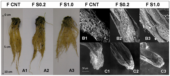
Yield responses depend on whether water distribution was limiting. In lettuce, the nonionic surfactant improved nutrient use efficiency but did not increase marketable yield under well-watered conditions. Quality can benefit: lettuce fertigated with a nonionic methyl-oxirane surfactant at ~1000 ppm showed a significant reduction in leaf nitrate accumulation compared with controls, alongside indications of shallower, more uniform wetting of the upper root zone (6).
Persistence and accumulation
Repeated use matters. In sand models, a polyoxyalkylene polymer surfactant (PoAP) sorbed to particles and increased hydrophobicity after repeated applications, whereas an alkyl block polymer (ABP) maintained or improved wettability and did not leave a hydrophobic residue. Chemistry dictates long-term behavior, so product choice is critical (4).
Toxicity
There is a hard ceiling for some agents. Hydroponic lettuce exposed to the anionic detergent Igepon showed acute root damage at ≥250 ppm, with browning within hours and growth suppression, although plants recovered after the surfactant degraded in solution (5). Practical takeaway: avoid harsh anionic detergents and keep any surfactant well below known toxicity thresholds.
Tables
Table 1. Water behavior in soilless substrates after root-zone wetting agents
Acute root phytotoxicity at and above 250 ppm; recovery after degradation of the agent
Practical rates
In closed hydroponic or recirculating fertigation, start conservatively. Research showing benefits without injury typically used ~50–1000 ppm, with several studies centering on ~1000 ppm weekly pulses in drip systems, or ~200–1000 ppm continuous-equivalent dosing in trials on leafy greens (3)(6). Very low concentrations can already fix wettability issues, as the 2 ppm result illustrates (1). Always monitor for foaming, root browning, or oily films. Avoid cationic disinfectant-type surfactants at the root zone and keep anionic detergents far below the 250 ppm lettuce toxicity threshold (5). Choose chemistries that do not accumulate with repeated use (4).
Conclusion
For soilless production, exogenous root applications of wetting agents are a precise way to restore uniform wetting, stabilize nutrient delivery, and improve nutrient use efficiency. Expect neutral yield when irrigation is already optimal, but better quality in leafy greens via lower leaf nitrate, and less nutrient loss in drain when media are reused or prone to channeling. Use the lowest effective ppm, prefer nonionic chemistries validated in horticultural systems, and be wary of products that persist or sorb to media. Done right, wetting agents are a small, high-leverage tweak that keeps the entire root zone working for you, not against you.
Root-applied auxins in hydroponics: where they help, where they don’t
Introduction
Auxins can modulate root architecture, fruiting and stress responses. In hydroponic and substrate soilless systems, exogenous root-zone applications at very low ppm sometimes boost yield or quality. Push the dose and you flip the response. Below I review peer-reviewed work on widely grown crops, focusing on species, timing, exact dosages converted to ppm, and toxic thresholds. Where possible I prioritize reviews to frame context, but yield data come from primary trials.
Model representation of the NAA molecule, a very commonly used auxin in plant culture.
Evidence & discussion
Sweet pepper. Two lines of evidence exist. First, fertigation with a commercial IBA product at 0.4 percent active (4000 ppm in the stock) applied weekly from early fruit development at 0.5 L ha⁻¹ outperformed 1.0 L ha⁻¹, increasing marketable yield while improving root mass and water and nutrient uptake in perlite culture (1). Second, a separate trial compared root fertigation vs foliar using a formulation containing 6.75 g L⁻¹ NAA and 18 g L⁻¹ NAA-amide. The fertigation rate was 0.6 mL L⁻¹ of product in the solution, equal to ~4 ppm NAA plus ~10.8 ppm NAA-amide per application; foliar used 0.4 mL L⁻¹ or ~2.7 ppm NAA plus ~7.2 ppm NAA-amide. Early and total yield were higher with fertigation, while foliar favored some quality traits like firmness and soluble solids (5). Practical read: peppers respond to root-zone auxin in the single-digit ppm range, but more is not better.
Melon. The same IBA approach that helped pepper flopped in melon. In perlite greenhouse culture, 0.4 percent IBA applied weekly at 0.5 or 1.0 L ha⁻¹ did not improve yield or water or nutrient relations. Authors concluded it is not an effective tool for commercial melon in soilless culture (2). Species matter.
Strawberry. In long recirculating systems, autotoxic phenolics depress growth and fruiting. A one-time root or crown dip in NAA before transplant at 5.4 μM NAA, which is ~1 ppm, mitigated autotoxicity and restored flower and fruit numbers compared with untreated plants. A higher 54 μM dose, about 10 ppm, was less effective (3). Timing was everything.
Toxic thresholds from hydroponic seedlings. While not a yield trial, maize in nutrient solution shows the margins. IBA at 10⁻¹¹ M is ~0.000002 ppm and stimulated root growth, but 10⁻⁷ M is ~0.02 ppm and significantly stunted primary root elongation and biomass. The same hormone switches from helpful to harmful across four orders of magnitude (4). That narrow window explains why melon trials can miss and pepper trials can hit. For broader context on root-zone biostimulation via fertigation programs, see this review (6).
Tables
Table 1. Positive responses to exogenous auxin at the root zone in soilless crops
Crop & system
Auxin and delivery
Dose in root zone (ppm)
Timing
Outcome
Sweet pepper, perlite
IBA 0.4 percent product via fertigation
Stock is 4000; applied 0.5 L ha⁻¹ weekly
From early fruit development
Higher marketable yield at 0.5 vs 1.0 L ha⁻¹; improved root mass and water and nutrient uptake (1)
Sweet pepper, soilless
NAA + NAA-amide via fertigation
~4 NAA + ~10.8 NAA-amide per application
Weekly during production
Higher early and total yield vs foliar; foliar favored firmness and °Brix (5)
Strawberry, recirculating hydroponics
NAA root or crown dip
~1 optimal; ~10 less effective
One time at transplant
Mitigated autotoxic yield loss; restored flower and fruit counts under closed reuse (3)
Table 2. Null results and toxic thresholds
Crop or context
Auxin & delivery
Threshold or tested dose (ppm)
Timing
Result
Melon, perlite greenhouse
IBA 0.4 percent via fertigation
Stock 4000; 0.5 or 1.0 L ha⁻¹ weekly
Season-long
No improvement in yield or water or nutrient relations (2)
Maize seedlings, hydroponic assay
IBA in solution
0.000002 stimulatory vs 0.02 inhibitory
Continuous exposure
Root growth stimulation at ultra-low ppm but marked stunting by 0.02 ppm(4)
Conclusion
Root-applied auxins are not a silver bullet. They can raise yield or preserve quality, but only when dose and timing line up with the crop’s physiology. Peppers respond to single-digit ppm root fertigation with higher early and total yields, while melons do not. Strawberries benefit from a ~1 ppm pre-plant dip that preempts autotoxicity, whereas ~10 ppm underperforms. Hydroponic seedling work reinforces the risk: ~0.02 ppm IBA already suppresses maize roots. The safe play is to trial low, crop-specific ppm near published values, apply at the stage that matters, and stop if marketable yield does not move. If you treat auxins like a nutrient and “turn them up,” they will punish you. If you treat them as a precise signal, they can pay off.
How to easily lower the costs of your Athena nutrient regime
You can make your Athena schedule much cheaper by replacing the pH up products with simple raw salts. Branded pH management and buffering products like Athena Balance and Athena Pro Balance are, at their core, just sources of potassium bases delivered in carbonate or silicate form. They are however, very over priced for what they are and can be a high percentage of the overall cost of running these nutrient regimes. By understanding their labels and safety data sheets, we can replicate these formulations with commodity salts, achieving equivalent nutritional and pH adjusting outcomes at a fraction of the cost.
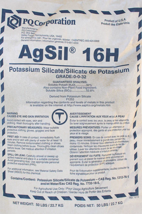
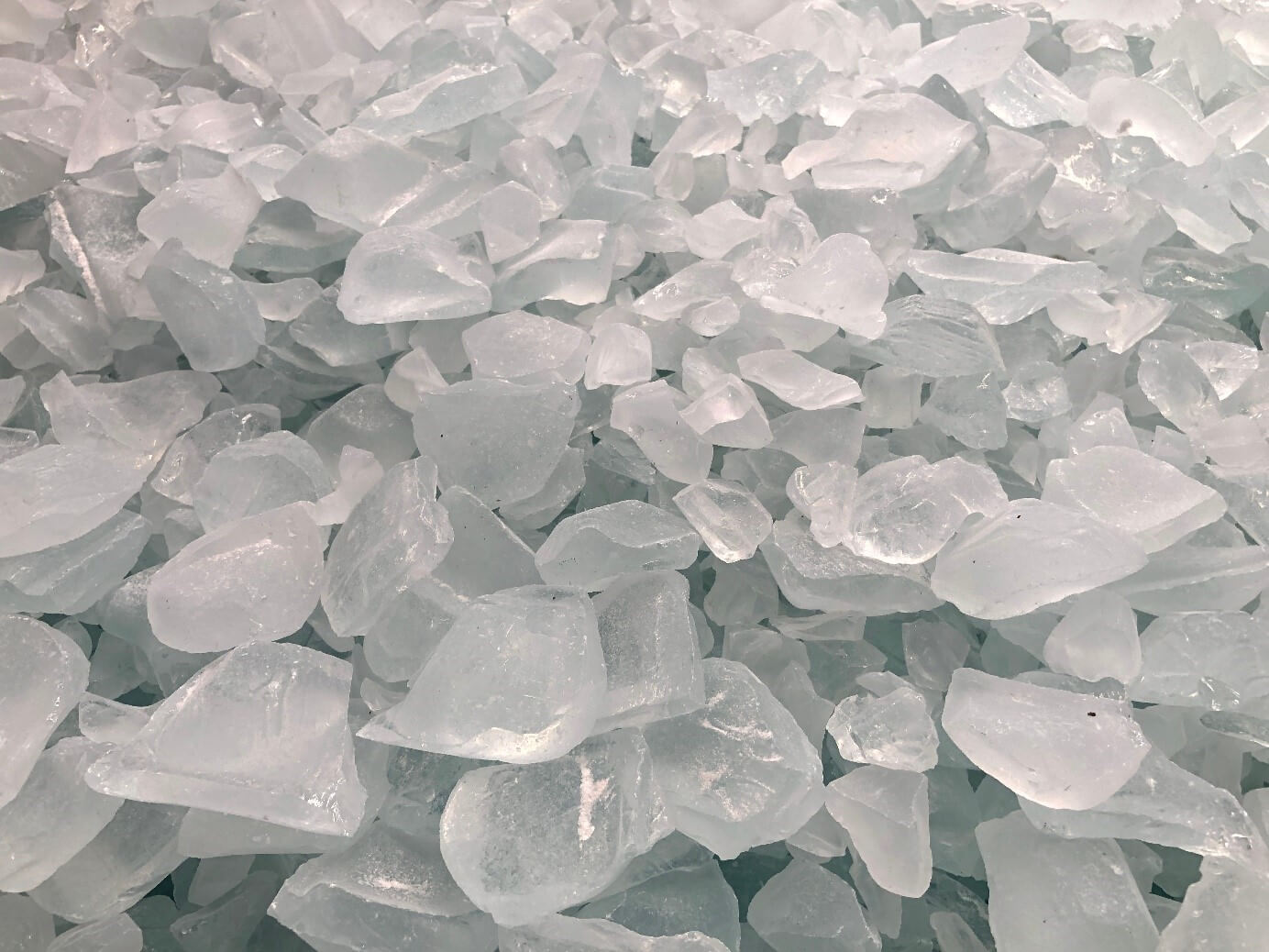
AgSil 16H, a very common base used to prepare potassium silicate solutions.
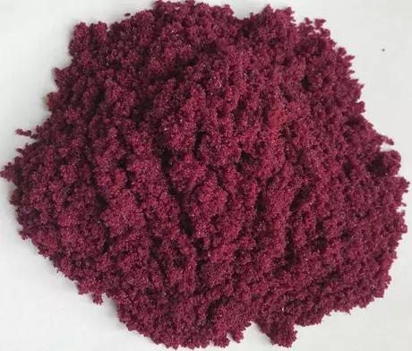
Athena Pro Balance can be replaced with Potassium Carbonate The powdered Pro Balance product is likely nothing more than high-purity potassium carbonate (K₂CO₃), usually 98.5–100% pure. Chemically, K₂CO₃ contains ~68% K₂O-equivalent by weight, which is exactly what the Athena Pro Balance label reflects. This means you don’t need to blend or dilute anything to make a replacement, simply sourcing food-grade or fertilizer-grade potassium carbonate is sufficient. You can dose it directly as you would the branded powder, bearing in mind it is strongly alkaline and should be added to water with care. Storage should be in sealed HDPE containers to avoid caking from atmospheric moisture.
Athena Blended Balance (liquid) can be replaced with an AgSil 16H solution The liquid Balance label shows 2% K₂O. AgSil 16H, a common potassium silicate source, contains 32% K₂O and ~53% SiO₂. To reproduce the K₂O content of Athena Balance, you need to dilute AgSil at the correct ratio:
Target is 2% K₂O.
Required fraction = 2 / 32 = 0.0625.
This means 6.25% (w/w) AgSil in water.
Translated to a practical recipe, this equals 236.6 g of AgSil 16H per US gallon of solution (3.785 L), topped up with RO water (must be RO or distilled water). Dissolve the AgSil slowly with vigorous mixing, as potassium silicate is highly viscous and alkaline. The result is essentially identical in potassium concentration to the branded Balance, with the added benefit of supplying soluble silica (~1.55% Si in the solution).
Improving stability with KOH One common issue with potassium silicate solutions is their tendency to polymerize or precipitate over time, especially at lower concentrations or in the presence of divalent cations. To mitigate this, adding a small amount of potassium hydroxide (KOH) helps maintain a strongly alkaline environment that discourages silica gelation. For the recipe above, adding 1 g of KOH per gallon of solution is a simple way to improve stability during storage. This will not significantly change the K₂O content but will keep the solution more stable and easier to handle.
Cost Analysis Beyond the chemistry, cost is the main driver for making these substitutions. Let’s look at a ballpark comparison based on typical retail prices (USD, 2025):
Product
Retail Price
Equivalent Raw Material
Raw Material Price
Cost per Gallon of Finished Equivalent
Athena Pro Balance (powder)
~$7 per lb
Potassium carbonate
~$2 per lb
Replacement is more than 3x cheaper
Athena Balance (liquid)
~$20-40 per gallon
AgSil 16H + 1 g KOH
~$6.4 per lb AgSil, ~$5 per lb KOH (~3$ AgSil + 1c of KOH per gal)
Replacement costs is around 10x cheaper
For the Balance liquid in particular, the price difference is striking: the branded gallon runs around $20-40, while the equivalent solution made from AgSil 16H plus a pinch of KOH comes out to under $3 per gallon, even at retail chemical pricing. The Pro Balance substitution is less dramatic in absolute terms but still represents substantial savings over time.
Take-home message Replacing Athena Pro Balance is as simple as sourcing potassium carbonate, while Athena Balance can be reliably reproduced with a potassium silicate solution prepared from AgSil 16H plus a small stabilizing addition of KOH. For growers comfortable working with raw salts, this substitution strategy provides full control, predictable composition, and significant cost savings while providing a drop-in replacement for one of the most expensive parts of the Athena nutrient line.
Chitosan in hydroponic and soilless crops: what actually works
In hydroponic and substrate systems chitosan can help, but only inside fairly narrow windows of dose, molecular traits, and crop context. Here is what the strongest hydroponic and soilless evidence shows for common greenhouse crops, with doses in ppm and forms that have actually been tested in peer-reviewed trials.
Chitosan powder, used as a biostimulant in soilless cultivation
What matters before you dose
Form and solubility. Most horticultural studies use acid-solubilized chitosan, typically chitosan acetate prepared by dissolving chitosan in dilute acetic acid. Solubility improves as degree of deacetylation increases and molecular weight decreases. That changes biological activity and leaf penetration, which is why not all chitosans behave the same in crops grown without soil. Review data across crops confirms that activity depends on origin, degree of deacetylation, molecular weight and derivative used, not just “chitosan” on the label (1).
Degree of deacetylation and molecular weight. Higher deacetylation increases positive charge density and solubility in the acidified sprays most growers use. Lower to mid molecular weight generally penetrates tissues better; very high molecular weight tends to act more at surfaces. Reviews focused on crop plants note these relationships and explain why different products show inconsistent results if DD and MW are not controlled (1).
Application route. Foliar and rootzone applications are not interchangeable. Foliar sprays in hydroponics commonly use 50 to 200 ppm for stress mitigation and quality endpoints. Rootzone dosing inside recirculating solutions can work for disease suppression at similar or higher ppm, but the tolerance window is tighter and crop-dependent. A 2024 root-focused review flags that root exposure can inhibit growth if dose and MW are off, even while defense responses go up (2).
Source. Commercial material is generally crustacean-derived, with fungal-derived chitosan available at smaller scale. Origin mainly matters through DD, MW and impurities like ash and protein. Again, agronomic performance maps back to those properties rather than source alone (1).
What the hydroponic and soilless studies actually show
Leafy greens and fruiting vegetables most tested in soilless settings
Lettuce, deep-flow hydroponics, foliar. In a controlled deep-flow system, foliar chitosan at 100 ppm mitigated salt stress, improved relative water content and chlorophyll, and reduced membrane damage markers. The trial used exogenous chitosan applied to leaves while plants grew in circulating nutrient solution, so the result is directly relevant to recirculating NFT or DFT growers (3).
Cucumber, hydroponic rootzone, disease control. In a classic hydroponic study, adding 100 to 400 ppm chitosan to the nutrient solution suppressed Pythium aphanidermatum root rot and induced host defenses without visible phytotoxicity at those doses. This is one of the best-controlled demonstrations of rootzone efficacy in a soilless system (4).
Tomato, soilless substrate, chitosan-based material at the rootzone. A soilless peat and perlite greenhouse system received a chitosan polyvinyl alcohol hydrogel with copper nanoparticles placed in the rootzone. The treatment improved growth, antioxidant capacity and yield relative to the untreated control. This is not a simple chitosan salt spray and the dose was delivered as a solid material rather than a ppm solution, but it shows chitosan-based materials can be integrated into substrate programs in practice (5).
Context across crops. A comprehensive review of chitosan for plant protection and elicitation explains the defense activation seen above and why responses are dose and MW dependent. It also documents successful use patterns that generalize to greenhouse crops treated by foliar or root routes (6).
Practical dose ranges that align with the hydroponic evidence
If you want the odds on your side in hydroponics or inert substrates, stay inside these lanes and confirm on a small block first.
Foliar, leafy greens and fruiting vegetables in hydroponics or inert substrate. 50 to 150 ppm per spray, usually every 7 to 10 days around stress periods. The deep-flow lettuce result sits at 100 ppm and delivered physiological benefits under salinity (3).
Rootzone, recirculating hydroponics. 100 to 400 ppm in the circulating solution only when you have a clear disease target like Pythium in cucumber. For general biostimulation, root dosing is higher risk. The hydroponic cucumber study used 100 and 400 ppm to suppress Pythium effectively (4). Outside this range you are more likely to see growth penalties than benefits according to root-focused syntheses (2).
Chemistry targets when purchasing. Prefer DD around 80 to 90 percent and low to mid MW material for foliar work. Verify supplier certificates rather than marketing bullets. The crop reviews explaining DD and MW effects are clear that these traits determine outcomes (1).
Summary tables
Table 1. Trials in hydroponic or soilless systems with chitosan
Crop
System
Application route
Chitosan form
Dose used (ppm)
Reported effect
Reference
Lettuce
Deep-flow hydroponics
Foliar spray
Acid-solubilized chitosan solution
100
Mitigated salinity stress, higher RWC and chlorophyll, lower oxidative damage
Pathogen suppression in roots and elicitation of defenses
Risk profile
Low when DD and MW are appropriate and pH is controlled
Higher. Dose and MW errors can reduce root growth and yield
Evidence base in soilless settings
Deep-flow lettuce shows clear physiological benefits at 100 ppm (3)
Hydroponic cucumber shows robust Pythium control at 100 to 400 ppm (4)
How to deploy without shooting yourself in the foot
Start with foliar at 100 ppm on a small block. If your chitosan is low to mid MW and 80 to 90 percent DD, you are in the same ballpark as the effective lettuce hydroponic protocol (3).
Reserve root dosing for disease pressure. If you are chasing Pythium in cucumber, 100 to 400 ppm in the solution is supported. For general “growth promotion”, root dosing is more likely to backfire than help in recirculating systems (4), (2).
Verify product specs. Ask for DD and MW. If the vendor will not provide them, find one who will. The variability you see in practice maps to those two numbers (1).
Do not stack unknowns. Mixing chitosan with copper, acids, or surfactants without a clear recipe can change activity. That can help in substrate programs where materials are embedded, as in the hydrogel example, but it is not a blank check (5).
Measure the outcome that pays. Run a side-by-side block with your limiting stress in view. If you cannot tie chitosan to a measurable gain in yield, quality or loss avoidance in your system, move on. Elicitation without payoff is just cost (6).
Iodine in Hydroponic Crops: An Emerging Biostimulant
Introduction
Iodine sits in a weird spot in plant nutrition. It is essential for humans, not officially essential for higher plants, yet low, well chosen doses often push crops to perform better in controlled systems. The key is dose and form. Get either wrong and you tank growth. Get them right and you can see yield and stress-tolerance gains that are economically meaningful. Recent reviews lay out both the promise and the pitfalls, so let’s cut through the noise and focus on agronomically relevant hydroponic and soilless work only. (1)
Potassium iodide, one of the most common forms used to supplement iodine in hydroponic culture.
Why iodine can behave like a biostimulant
Mechanistically, iodine at trace levels appears to influence redox balance and stress signaling and can even become covalently bound to plant proteins. Proteomic evidence has shown widespread protein iodination, and plants deprived of iodine under sterile hydroponics grow worse until micromolar-range iodine is restored. That does not make iodine “essential” in the strict sense, but it explains why tiny doses can trigger outsized responses. (2)
Form matters
Across multiple hydroponic tests, iodide is absorbed faster and is more phytotoxic than iodate. In basil floating culture, growth was unaffected by roughly 1.27 ppm iodine as KI or 12.69 ppm iodine as KIO3, but KI above about 6.35 ppm iodine cut biomass hard, while KIO3 needed far higher levels to do the same. That is a practical takeaway for nutrient solution design. Favor iodate when you are exploring a new crop or cultivar. (3)
Evidence from hydroponic and soilless crops
Lettuce
A classic water-culture study ran 0.013 to 0.129 ppm iodine in solution and saw no biomass penalty while leaf iodine rose predictably. Iodide enriched tissue more than iodate at equal iodine, which is useful if your target is biofortification, not just a biostimulant effect. (4)
Under salinity, iodate becomes more interesting. In hydroponic lettuce with 100 mM NaCl, about 2.54 to 5.08 ppm iodine as KIO3 increased biomass and upregulated antioxidant metabolism, which is exactly what you want in salty recirculating systems. Push higher and the benefits fade. (5)
Strawberry
Hydroponic strawberry responded to very low iodine. Iodide at or below 0.25 ppm and iodate at or below 0.50 ppm improved growth and fruit quality, while higher levels reduced biomass and hurt fruit quality metrics. You do not have much headroom here. (6)
Basil
Greenhouse floating culture trials on sweet basil showed cultivar-specific tolerance but the same pattern every time. KI starts biting growth above single-digit ppm iodine, while KIO3 is far gentler at comparable iodine. Antioxidant capacity trends are cultivar dependent, so do not generalize “more phenolics” as a guarantee of better growth. (7)
Tomato
Tomato is where yield effects get real. In growth-chamber work, fertigation with iodate at roughly 6.35 to 12.69 ppm iodine increased fruit yield by about 30 to 40 percent in a small-fruited cultivar. In a greenhouse trial with a commercial hybrid, much lower iodine in solution, around 0.025 to 1.27 ppm as KIO3, still improved plant fitness and mitigated part of the salt penalty. Dose tolerance depends on the system and the genotype, so copy-pasting numbers between cultivars is a bad idea. (8)
Cabbage
Hydroponic Chinese cabbage tested 0.01 to 1.0 ppm iodine as KI or KIO3. Uptake and partitioning behaved differently by species and form. The practical read is that both forms work for biofortification within that band, but I would still lean iodate first for safety. (9)
Working ranges seen in hydroponic or soilless trials
Crop
System
Iodine form used
Dose range tested in literature (ppm as I)
Observed direction of effect
Lettuce
Water culture
Iodide and iodate
0.013 to 0.129
Neutral on biomass, strong tissue enrichment at all doses tested
Lettuce under salinity
Hydroponic with 100 mM NaCl
Iodate
~2.54 to 5.08
Biomass increased, antioxidant system activation
Strawberry
Hydroponic
Iodide and iodate
Beneficial at or below 0.25 (I−) and 0.50 (IO3−)
Growth and fruit quality improved at low doses, declines above
Basil
Floating culture
Iodide and iodate
Safe near 1.27 as KI, 12.69 as KIO3; toxicity above ~6.35 as KI
KI far more phytotoxic than KIO3 at equal iodine
Tomato
Substrate fertigation and growth chamber
Iodate
~0.025 to 12.69 depending on setup
Yield and stress tolerance improved within study-specific bands
Cabbage
Hydroponic
Iodide and iodate
0.01 to 1.0
Both forms accumulated; response form-dependent
Practical setup that does not wreck a crop
Start with iodate. It is consistently less phytotoxic in solution culture than iodide at the same iodine level. Use iodide later only if you have a clear reason. (7)
Leafy greens Conservative exploratory band: 0.03 to 0.10 ppm iodine in solution during vegetative growth. If you are running saline conditions, you can test up to about 2.5 to 5.1 ppm as iodate for stress mitigation, but do not do this blind outside a salinity trial. (4)(5)
Strawberry Keep solution iodine low. Try 0.05 to 0.25 ppm as iodide or 0.10 to 0.50 ppm as iodate. Expect quality shifts alongside biofortification, and expect penalties if you push higher. (6)
Basil If you work with KI, do not exceed about 1.3 ppm iodine without a reason and tight monitoring. With KIO3, you have more headroom, but benefits are not guaranteed at the higher end. (7)
Tomato In substrate systems, exploratory fertigation bands that have shown positive responses run roughly 0.025 to 1.27 ppm iodine as iodate for commercial cultivars. Higher doses around 6.50 to 12.50 ppm have improved yield in small-fruited genotypes under controlled conditions, but those are not starting points for a commercial house. (8)
Cabbage and other Brassicas 0.01 to 1.0 ppm works for biofortification trials in solution culture. Track form-specific uptake. (9)
Common failure modes
Using iodide when you should have used iodate. Iodide is more phytotoxic in water culture. If you switch to iodide, cut the ppm accordingly and watch plants closely. (7)
Copying doses between crops or between stress contexts. Lettuce under salt stress tolerated and benefited from multi-ppm iodate that would be overkill in non-saline runs. (5)
Chasing biofortification at the expense of growth. Strawberry is very sensitive; the window for improvement is narrow and easy to overshoot. (6)
Assuming universality. Tomato shows real yield gains, but the best range depends on cultivar and system. Validate locally. (8)
Crop
Best form to start
Trial band to test next (ppm as I)
Notes you should not ignore
Lettuce
KIO3
0.03–0.10 for routine runs; up to 2.5–5.1 only in salinity trials
Tissue enrichment is easy at sub-ppm; benefits need stress context
Strawberry
KI or KIO3
0.05–0.25 as KI; 0.10–0.50 as KIO3
Quality improved at low levels; penalties above
Basil
KIO3
0.5–3.0
KI becomes risky above low single digits
Tomato
KIO3
0.025–1.27 in commercial substrate; leave 6.5–12.5 to controlled trials
Verify by cultivar; watch fruit quality metrics
Cabbage
KIO3
0.05–0.5
Uptake is efficient; track partitioning by organ
Final word
Iodine can behave like a biostimulant in hydroponics and soilless systems, but only if you respect its razor-thin margin between helpful and harmful. Start small, prefer iodate, and validate on your own cultivars and systems instead of trusting a one-size-fits-all recipe. If you need a broader framework for running precise biofortification trials in soilless production, recent reviews are clear about why controlled systems are the right place to do this work. (9)
Cobalt in hydroponics as a biostimulant
People ask about dosing cobalt in recirculating systems to “stimulate” growth or flowering. For the crops that matter in hydroponics and soilless culture, peer-reviewed work does not show reliable growth or yield benefits from adding cobalt to the solution. What the literature does show is straightforward: cobalt is readily taken up at low ppm, it inhibits ethylene biosynthesis at pharmacological doses, and it becomes toxic fast when you push concentration. The burden of proof for agronomic benefit is still unmet. Below I summarize what high-quality studies in hydroponics and soilless systems actually report.
cobalt (II) chloride, the most common form of chloride used in studies
What cobalt does in plants
Cobalt is not established as essential for most higher plants. It is essential for N-fixing microbes and therefore matters in legumes, but for tomato, cucumber, lettuce and the like, its status is “potentially beneficial at very low levels, toxic at modest excess.” A recent review frames this clearly and compiles transport and toxicity data across species (Frontiers in Plant Science, 2021).
A second, practical point is mechanism. Cobalt ions inhibit ACC oxidase, the last step in ethylene biosynthesis. That is why physiologists use cobalt chloride in short, high-dose treatments to suppress ethylene responses in experimental tissues. Classic work documents this inhibition in cucumber and other plants (Plant Physiology, 1976).
Ethylene inhibition can, in principle, delay senescence or alter stress signaling. The catch is dose. The amounts that clearly block ethylene in lab tissues are usually far above what you want sloshing around a long-cycle greenhouse system, and benefits rarely translate to whole plants under production conditions.
What happens in hydroponics and soilless systems
Tomato
Nutrient solution exposure, subtoxic range Tomato grown hydroponically with cobalt at 0.30 ppm and 1.18 ppm showed strong root retention and limited shoot transfer. This is uptake behavior, not a biostimulant response, and the authors did not report yield benefits. The forms used were cobalt(II) salts in solution culture (Environmental Science & Technology, 2010).
Toxicity under higher exposure A hydroponic study imposed severe cobalt stress at 23.57 ppm and observed depressed biomass, disrupted water status, chlorophyll loss and oxidative damage in tomato. Cobalt was supplied as cobalt chloride in the nutrient media. Plant growth regulators mitigated symptoms but did not make cobalt itself beneficial (Chemosphere, 2021).
Lettuce
Toxicity in greenhouse hydroponics with inert media Iceberg lettuce grown in a perlite based hydroponic system suffered growth and pigment losses at 11.79 ppm cobalt. Cobalt was added as cobalt salt to a modified Hoagland solution. The same paper showed nitric oxide donor treatments could blunt the damage, which again argues cobalt at this level is a stressor, not a stimulant (Chilean Journal of Agricultural Research, 2020)
Cucumber
Mechanistic ethylene work, not production benefit Multiple peer-reviewed studies in cucumber use cobalt chloride as an ethylene biosynthesis inhibitor in explants or short assays. These demonstrate the mechanism but are not agronomic validations for dosing cobalt into a recirculating system for weeks (Plant Physiology, 1976; Forests, 2021).
Summary table of relevant studies in hydroponics and soilless culture
Significant growth and pigment losses at this dose; NO donor partially mitigated damage. Chilean J. Agric. Res. 2020
Cucumber
Short mechanistic assays
Cobalt chloride
used as ethylene inhibitor in short assays
Explants or detached tissues
Confirms ethylene inhibition by Co²⁺; not a production recommendation. Plant Physiology 1976
So is cobalt a biostimulant in hydroponic vegetables
For tomato, cucumber and lettuce grown hydroponically or in soilless culture, peer-reviewed journal data do not support cobalt as a legitimate biostimulant input. You can inhibit ethylene transiently with cobalt chloride in lab tissues, but that is not a recipe for higher yield in a recirculating system. The agronomic studies that actually dose solutions show either neutral responses at sub-ppm levels or clear toxicity when you push into low double digits. The general biology context from a recent cobalt review matches this picture and does not contradict it (Frontiers in Plant Science, 2021).
Practical guidance for hydroponic and soilless growers
Default practice Do not add cobalt intentionally to non-legume hydroponic recipes. There is no reproducible benefit and real risk of toxicity in the low tens of ppm, with lettuce showing damage already at ~12 ppm and tomato at ~24 ppm under hydroponic conditions. (see here, or here)
If you want to experiment Keep total cobalt in solution at sub-ppm levels and treat it as a research trial, not a production strategy. Track solution cobalt with ICP if you can. The only peer-reviewed hydroponic tomato data near this range are 0.30 to 1.18 ppm, which documented transport behavior, not stimulation.
Forms used in the literature Cobalt chloride is the dominant form when researchers test ethylene inhibition or impose cobalt stress. Cobalt sulfate also appears in some soilless protocols. Neither form has peer-reviewed evidence of yield stimulation in hydroponic tomato, cucumber or lettuce. (see here or here)
Legumes are the exception Cobalt matters indirectly via N-fixing symbionts. If you are growing legumes in soilless systems, cobalt management belongs in the microbial nutrition discussion, not as a general biostimulant for non-legumes (see here).
Not defined for production, lab tissues often use high short-term doses
CoCl₂ used to block ethylene in explants; not a production recommendation. Plant Physiology 1976
Bottom line
If you grow tomato, cucumber or lettuce in hydroponics or inert media, cobalt is not a proven biostimulant. At sub-ppm levels you might see nothing. Push it into the low tens of ppm and you will see toxicity. The only unequivocal “effect” you can count on is ethylene inhibition during short, high-dose laboratory treatments with cobalt chloride, which is not a safe or sensible production tactic. Until robust, peer-reviewed hydroponic trials show yield or quality gains at practical ppm, the rational move is to leave cobalt out.
Common questions about silicon in nutrient solutions
Introduction
We know that silicon can be a very beneficial element for many plant species (see some of my previous posts here and here). It mainly enhances disease resistance and increases the structural integrity of plant tissue. Because of these advantages, you will want to add silicon to your nutrient solution. However, there are a lot of misconceptions and questions about the use of Si in plants and the exact form of Si that you should use. In this post I am going to address some of the most common questions about silicon sources and how to use them properly.
Alkali metal silicates are the most common sources of soluble silicon used. They also have the lowest cost by gram of Si.
What sources are available?
To use silicon in nutrient solutions, we will generally have 3 types of sources available.
First, we have basic potassium silicates, which are solids or solutions derived from the reactions of silica with potassium hydroxide. In this category you have popular products like AgSil 16H and liquid concentrates like Growtek Pro-Silicate. These products have a very basic pH.
Second, we have acid stabilized silicon products. These are products like PowerSi Classic and OSA28. These products are always liquids and contain monosilicic acid in an acidic environment, with stabilizing agents added to prevent the polymerization of the monosilicic acid.
Third, we have non-aqueousproducts with organosilicon reagents, like Grow-Genius. These products do not contain water and are derived from reagents like TEOS (tetraethyl ortho-silicate) and other Si containing compounds, mainly Si containing surfactants. They are not in forms that are plant available but will generate these forms when in contact with water.
Do potassium silicates contain “less available” silicon?
When you dissolve a potassium silicate at high concentration, it forms silicate oligomers. These are large silicon chains that get stabilized in basic solutions because of their high negative charge. This is why you can create highly concentrated potassium silicate solutions in basic pH. As a matter of fact, making the solutions more basic with added potassium hydroxide often enhances the solubility of potassium silicate solids like AgSil16H (see here for a procedure on how to do this). However, when the molar concentration decreases the silicate hydrolyzes into monomeric silicate anions.
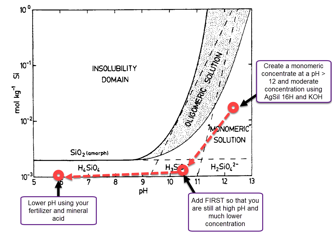
Original background image taken from here. To create a monomeric solution you need high pH and low concentration. Then you lower the pH to get to monosilicic acid.
When potassium silicate is diluted in nutrient solutions, this is exactly what happens. The reduction in concentration hydrolyzes the Silicates into monomers. If the solution pH is then lowered, the final form present will be monosilicic acid. If you properly prepare a nutrient solution with potassium silicate, the end form will be monosilicic acid, the form that is mostly available to plants.
It is a misconception that potassium silicates are somehow less “plant available”. They end up producing monosilicic acid and being perfectly available, when used properly.
How do I properly use a potassium silicate?
First, if using a solid, you need to prepare a stock solution no more concentrated than 45g/L. The recommendation with AgSil 16H would be to prepare a stock solution at 15g/gal and then using this solution at a rate of 38mL/gal of final solution (injection rate of 1%). To increase the stability of your AgSil 16H concentrate you can add 1g/gal of KOH. The end addition to your solution will be +9.8ppm of Si as elemental Si and +11.55ppm of K. The KOH addition and low 15g/gal concentration ensures that silicate will already be largely present as monomeric silicate anions.
Second, make sure to add this solution to your water first. If you add this solution after nutrients, the Si will come into contact with Ca and Mg in its concentrated form, which will cause problems with its stability in solution. Add it first, then add your lowest pH fertilizer concentrate, then your Ca containing concentrate, then finally decrease the pH with an acid to the desired level if needed.
This procedure ensures you get a final solution containing monosilicic acid that will be stable. If you increase the Si in the stock solution, change the injection order, or increase the Si in the end solution beyond 20ppm of Si as elemental Si you might end up with precipitated and unavailable Si forms.
Why would you use acid-stabilized Si products?
Acid stabilized silicon sources are not more plant available. However, their starting pH is usually low and their mineral composition can also be minimal (depending on the preparation process). This means they can lower the need for acid additions and can help lower the pH of hard water sources when used. They can also contain stabilizing agents that could be beneficial for plants. However, the exact stabilizers used and the exact mineral composition used will vary substantially by product, since there are a wide array of choices available to manufacturers.
In the end, at the pH where plants are fed, acid stabilized Si and potassium silicate sources generate the exact same monosilicic acid. Plant availability is not an advantage of using this sort of product.
Why would you use non-aqueous Si products?
These products can be much more highly concentrated than either basic silicon or acid stabilized liquid silicon products by mass. This is because they are made from Si forms that are highly stable under water-free conditions. This means you can buy a small amount and add a small amount to your reservoir per gallon of solution prepared. Another advantage is that they are pH neutral and do not alter the pH of nutrient solutions at all. The formation of the silicic acid from these products requires only reactions with water, so no mineral addition, stabilizer additions or pH modifications happen.
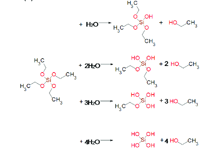
Reaction of TEOS with water to produce different silicic acids (plus ethanol)
A significant point however is that the reaction of a product like TEOS with water releases other substances into solution. For each 10 ppm of Si as elemental Si that you add from TEOS you will in fact be adding ~66pm of ethanol to your solution. These alcohols can be very detrimental for root and plant growth, reason why the use of these non-aqueous Si products needs to be carefully considered. When using a product containing non-aqueous Si sources, it’s important to consider that these substances can accumulate in your root zone and may cause problems. Which organics are present and whether they will cause problems will depend on the exact formulation. When using these organosilicon sources, passing the nutrient solution through a carbon filter to remove these organics before contact with plant roots would be ideal.
Is the final Si in solution from any product type more stable?
No, all three types of products, when used properly, will end up as stable monosilicic acid in your solution. The stabilizing agents in acid-stabilized products will be so dilute that any additional stabilizing effect will be relatively non-existent. If Si is dilute enough (<20ppm of Si as elemental Si), then it will be stable in solution indefinitely (I measured 5 weeks with no changes in concentration). At higher Si concentration, the Si will tend to polymerize (no matter which source it comes from) which will create problems with stability. To have stable Si in solution make sure that you prepare it properly and that you keep the concentrations low enough.
If they are mostly the same in terms of Si availability, why do I see differences between different products at an equivalent Si application rate?
Despite all of the different Si products leading to the same form of Si in the final solution, acid-stabilized Si products will contain a wide array of additional substances that are going to be active nutritionally. For example, Boron and Molybdenum are very commonly used stabilizing agents. Products, like PowerSi bloom, also contain “exotic plant extracts” (according to their website). Commonly used stabilizing agents include glycerol, carnitine, choline and sorbitol. All of these could potentially have an effect on the plants at the concentrations added with these products. Some of these stabilizing agents are usually added at 10-50x the amount of Si present by mass, meaning that your Si supplement might be adding way more of these stabilizing agents than what you’re adding in terms of Si.
What product is more cost effective per delivered mole of monosilicic acid?
There is a lot of space in labeling regulations to allow fertilizer manufacturers to trick people into believing a product might be more concentrated or dilute than another. First of all, labeling a product as “% of monosilicic acid” does not mean that the product contains that percentage of monosilicic acid, it means that the product contains Si, such that if that silicon was all converted to mono-silicic acid, it would give that percent. The only products that contain monosilicic acid in its actual form from the start are acid-stabilized Si containing products, which are usually limited to low concentrations due to the reactivity of this molecule when present.
Both non-aqueous silicon products and soluble potassium silicate products contain precursors to monosilicic acid. One in the form of organosilicon compounds and the other in the form of silicate chains. As mentioned above, both precursors can lead to very high conversions to mono-silicic acid when properly used.
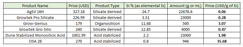
These prices were the lowest prices I could find for each product in Feb 2023. To find current prices, I suggest searching any products you’re interested in. Composition values taken are those provided by the manufacturer, converted to Si as elemental Si. Prices do not include shipping.
To compare the actual concentration of products, it is best to always convert the amounts to elemental Si percentage values. To convert monosilicic acid % values to Si, multiply the value by 0.2922, to convert SiO2 values to Si, multiply the value by 0.4674. For example, 40% Si as monosilicic acid is equivalent to 11.68% Si as elemental Si. Soluble potassium silicates like AgSil 16H can be around ~24% Si as elemental Si by mass, making them the most highly concentrated and lowest cost form of bioavailable silicon when used properly. More highly soluble potassium silicates than AgSil16H will usually be lower in Si, as higher K proportions lead to better solubility and a lesser need to add KOH when preparing stock solution. The table above, showcases the price differences per gram of Silicon of different products as of Jan 2023. When purchased in bulk (50 lbs) AgSil16H can be up to two orders of magnitude lower cost than other alternatives.
I have done lab tests measuring molybdenum reactive Si that show all the Si in AgSil16H can be quantitatively converted to monosilicic acid when following the preparation guidelines mentioned in this post.
What is your recommendation?
After studying the subject for years, using different products with different growers and testing the chemistry myself (preparing stabilized silicic acids and measuring active Si concentrations). Given the price of Si products and the chemistry involved, I would suggest anyone interested in Si supplementation in nutrient solutions to use a potassium silicate solid product. I would suggest to prepare a suitable stock with potassium silicate and potassium hydroxide to increase pH and stability and then prepare their nutrient solutions from dilutions of this stock. If a solid product like AgSil 16H is not available, then using a basic silicate concentrate product would be the next best choice. Usually preparing a more dilute stock from these products is recommended to ensure the stock already contains monomeric silicate.
I don’t think acid-stabilized silicon products or non-aqueous Si products are worth the price premium. If you’re having better results with a non-potassium silicate product compared to potassium silicate, bear in mind that this is likely because either the potassium silicate stock preparation and dilution were not done correctly or the product you’re using contains a substance different from Si that is giving you those effects. The stabilizing agents themselves are going to be much lower cost, so testing the eliciting effects of these agents might be more economical for you than using these expensive products long term.
In cases where mixing stocks and handling basic reagents is problematic or there is limited availability to adjust pH, then the use of non-aqueous Silicon reagents might be desirable. Non-aqueous silicon forms are also the most robust to mixing errors – wrong mixing order, mixing at variable pH, etc – because the hydrolysis reactions happen readily under a wide variety of conditions. However, my recommendation is to always couple these with carbon filtration to avoid potential issues from their organic side-products.
If you have issues with the use of soluble silicon sources – because of your initial water composition, injector limitations, cost, etc – and your media supports amending, I would also suggest considering using solid amendments to supplement Si (watch this video I made for more information). Amending can be a great choice, much more economical than soluble Si supplementation.
Do you have any questions about Si in nutrient solutions not addressed above? Feel free to leave a comment and I might also add it to the post!
A cost analysis of fertilizers for hydroponic/soilless growing in 2022
Why fertilizer costs matter
Fertilizer can be one of the largest expenses of a hydroponic growing facility. This is especially true when boutique fertilizers are used, instead of large scale commodity fertilizers. The use of non-recirculating systems with high nutrient concentrations also contributes heavily to high cost fertilizer usage. A medium scale growing facility working with boutique fertilizers can in some cases spend 2000-4000 USD per day. Even when using some of the most cost effective solutions, a facility can still spend 4000 USD per day if they use 20,000 gal/day with a nutrient line costing 0.2 USD/gal.
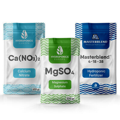
The above is a common combination of raw inputs and a standard blended input
In 2022, the high cost of energy and high inflation have increased raw fertilizer input costs to the highest point of the past decade, making the problem of fertilizer costs even more pressing. This has been specially the case for soluble phosphate fertilizers which have, in some cases, seen costs triple from the start of 2019. This is because soluble phosphates were largely produced in Russia and alternative sources of soluble phosphates had a hard time ramping up capacity at the same cost level as could be previously achieved.
To help people who are growing better assess their costs, I seek to paint a clear picture of the current cost level of commodity and boutique fertilizers as well as the cost levels that can be achieved with preparation of custom solutions.
Price sources
The cost analysis focuses on the US market. The prices I obtained for boutique fertilizers are from google searches where I found the cheapest costs at the highest scale I could find. For commodity fertilizers I used the price points of customhydronutrients.com, which is a trust-worthy website for the purchase of fertilizer inputs. These prices are also accessible from small to large scales, so they do not require large scales to be accessible. Boutique fertilizer companies might offer larger discounts to people who contact them directly to buy large amounts, but I did not use these prices as they are not publicly available.
To make comparisons easier, I will express all costs as costs per final gallon of nutrient solution, when prepared per the directions of the manufacturer or to arrive at formulations with a reasonable composition (formulations that can grow healthy, high yield crops). Please also note that I only considered fertilizers that could be used to prepare concentrated solutions to be used for injection, as these are fundamental to large scale growing operations. I also only considered powdered fertilizers as these offer the lowest cost. Liquid concentrated fertilizers – which are often substantially more expensive – were not considered.
For purposes of keeping the costs as low as possible I also only considered the base products from boutique fertilizer companies and did not consider the costs of any of their additives (line cleaners, boosters, hormones, etc). Shipping costs are also not considered here.
Blended fertilizers
The easiest, most accessible fertilizers for most people will be pre-blended fertilizers. Due to the proliferation of the cannabis industry, most of the pre-blended fertilizers that are sold to retail growers will be cannabis-centric and will have a considerably higher price than the blends currently used by the wider hydroponic industry.
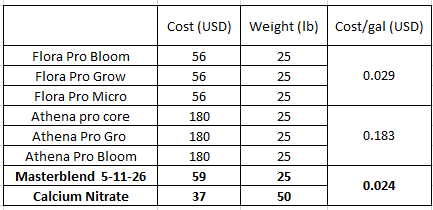
Table comparing a couple of boutique lines with a standard 5-11-26 preparation using a Masterblend product and Calcium nitrate.
The table above shows three representative fertilizer programs for comparison. The Flora Pro series from General Hydroponics was the lowest cost boutique fertilizer I could find, with a total cost of 0.029 USD per gallon at the recommended dosing rates by General Hydroponics. I also put the Athena line for comparison, as they often portray themselves as a low cost option for cannabis companies. Their cost is almost an order of magnitude higher, at 0.183 USD/gal. From this analysis it seems clear that their margins are much higher than those of General Hydroponics although they can be substantially more cost effective than other companies with even more expensive products.
After seeing the above table, it is clear that boutique companies are not price competitive against formulations using traditional blended fertilizers from the agricultural industry. A formulation using Masterblend 5-11-26 and Calcium nitrate, which could be perfectly adequate for the growth of flowering plants during their vegetative stage or purely vegetative plants like basil, has a cost of 0.024 USD/gal. Similar simple approaches using other blended products can be used to achieve a variety of compositions at a similar price tag.
Raw input fertilizers
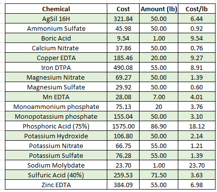
It is also interesting to consider the case of raw fertilizer inputs as this allows us to better think about formulations to reduce cost and also calculate whether making custom fertilizers is worth the expense. The table below shows you some commonly used bulk fertilizer inputs, their cost in USD and the cost per pound of each one of the products.
Cost and cost per pound of each fertilizer input
Micronutrients are the most expensive per pound, but since they are used at very low amounts, their total cost contribution to fertilizer solutions is often less than 0.002 USD/gal (not counting the iron). The cost of the bulk fertilizers is much more important from a cost impact perspective. From these fertilizers, potassium inputs are often the most expensive. Both potassium nitrate, potassium sulfate and monopotassium phosphate are usually large contributors to the total price of a hydroponic formulation. Soluble silicon amendments, like AgSil16H, are also often large contributors to the overall price of these formulations. The above analysis also shows that Phosphoric acid is a very expensive option for pH adjustments in hydroponics. For this reason – and a few other reasons out of the scope of this post – sulfuric acid should almost always be used.
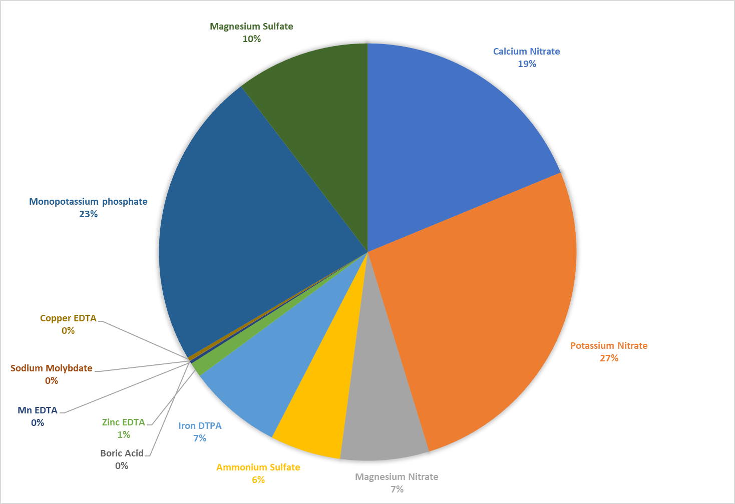
Cost contribution of bulk fertilizers to a custom hydroponic formulation.
The image above shows you the bulk contributions of all the raw inputs used in a sample custom formulation. The total cost of this formulation is around 0.016 USD/gal. If we supplemented Silicon from AgSil16H, the cost of this formulation would likely increase to close to 0.025-0.03g/gal depending on how much Si we would like to add. You can see here that the highest bulk costs are indeed the monopotassium phosphate and the potassium nitrate, it is unlikely that we would be able to diminish this cost contribution substantially, as this is the true bottom line of the fertilizer industry.
For most of my clients, formulation costs in real life will usually be between 0.01-0.03 USD/gal. The final cost will depend on which bulk discounts are available at scale, which plants the client is growing, what the cost of shipping the fertilizer is and which additional amendments beyond simple raw fertilization we choose to use. Sometimes, by using the nutrients already present in the water, substantial additional savings are possible with custom formulations.
Note that the above raw input analysis does not include the cost of labor to prepare the concentrated nutrients needed for injection. If a worker needs to spend a couple of hours per week mixing 25 gallons of each fertilizer then this, at 20 USD/hour, would likely increase the cost of the fertilizer by around 2-5%. Since workers can often mix batches of concentrated solutions that end up creating thousands of gallons of solution, the labor cost needed to mix fertilizers is often not meaningful relative to the overall cost of the inputs.
Balance between complexity and cost
From the above, it is clear that making your own fertilizer has the lowest cost, even at a small scale. However, it does add a substantial level of complexity to an operation and exposes the operation to a variety of potential mistakes dealing with preparation. A careful consideration of the advantages and disadvantages of mixing your fertilizer needs to be made. For large facilities, I believe this to be a no-brainer. At scale, it almost certainly makes sense to mix your own fertilizers.
However, it is true that at a medium scale, a grower might benefit from not doing their own mixing, as this simplifies their operation and allows them to focus on growing great plants while they grow. In this case, you can certainly – regardless of the plant you’re growing – create a formulation based on a widely available agricultural industry blend with perhaps one or two raw inputs, to achieve a highly cost effective formulation.
Of course, there is also an additional cost to fertilizer formulation, which – per the prices charged by myself and other colleagues – might cost you from hundreds to thousands of dollars depending on complexity. If you do not want to incur this cost, then you should bear in mind you will pay a perpetually higher price in your fertilizers, to a company that has done the formulation work for you.
At a large scale, you definitely do not want to go with a formulation that reduces the yield or quality of your plant product, so – if you lack the experience to do these formulations yourself – always make sure to hire someone who knows what they are doing.
In the simplest case, a formulation schedule of an agricultural preblended product – using for example the Masterblend 5-11-26 mentioned above – adjusted to your situation might lower your costs by an order of magnitude from an expensive boutique shop at a minimal increase in complexity and low formulation costs. Of course you can always make your own Masterblend proxy as a first step when you move to fully custom formulations. If it is not possible to use these types of blends – due to for example your water composition – a fully custom formulation will be required.
There is no reason to pay even higher prices
People in the traditional large scale hydroponic industry have been growing at very cost effective fertilizer prices for decades. If you are a small, medium or even large scale grower, there is no reason why your fertilizer costs should be astronomically high. There are no reasons to perpetually pay high margins to fertilizer companies and there is no reason why you shouldn’t take advantage of the easiest cost savings that can be achieved with products that are already available to the bulk agricultural industry. Now that the raw fertilizer input costs are even higher, it is more important than ever to go to lower cost methods to achieve your desired hydroponic formulations.
If you want to learn how to make your own fertilizers, then I advice you visit my youtube channel or read my blog articles on making your own fertilizers from raw inputs.
Are you using boutique fertilizers? Are you mixing your own? Please let us know about your experience in the comments below!
How to reuse your coco coir in soilless growing
Why reuse media
Buying new media and spending labor to mix, expand, and even amend it can be a costly process for growing facilities. Dumping media also involves going through a composting process, wasting nutrients that are already present in that media when it is thrown away. However, media in hydroponics serves a mostly structural role and there are no fundamental reasons why media like coco cannot be recycled and used in multiple crop cycles.
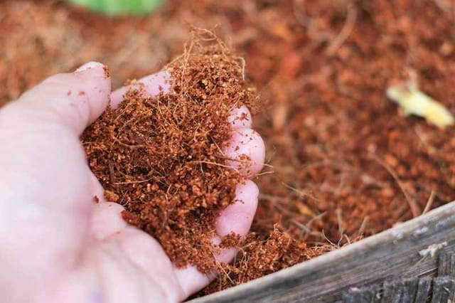
Coco coir commonly used as a substrate in soilless agriculture.
By reusing media, a grower can substantially reduce operational costs. This is because the media itself often contains an important amount of surplus nutrition and the roots and other organic components left behind by previous plants can also be used by new crops to sustain their growth. These added decomposing root structures also reduce channeling in the media and help improve its water retention as a function of time. After a media like coco is reused several times, the coco also degrades and becomes finer, further improving water retention.
Why media is often not reused
Reusing media is not without peril. When media is pristine, it is more predictable. You know its basic composition and you can feed it the same set of nutrients and hope to obtain very similar results. Nonetheless, after media goes through a growing cycle, its chemical composition changes and the starting point becomes much more variable. This means that a grower needs to somehow adjust nutrition to the changes in composition, which can often make it difficult for the crop to achieve consistent results.
If a grower reuses media but tries to feed as if the media was new, then problems with overaccumulation of nutrients in the media will happen and it will be hard for the grower to obtain reliable results. Reusing media requires a different approach to crop nutrition which scares people away because it strays from what nutrient companies and normal growing practices require. However we will now learn how media is chemically affected by cultivation and how we can take steps to reduce these effects and then successfully reuse it.
Media composition after a normal crop
In traditional coco growing, fertilizer regimes will tend to add a lot of nutrients to the coco through the growing cycle. From these nutrients, sulfates, phosphates, calcium and magnesium will tend to aggressively accumulate in the media while nutrients that are more soluble like nitrate and potassium will tend to accumulate to a lesser extent or be easier to remove.
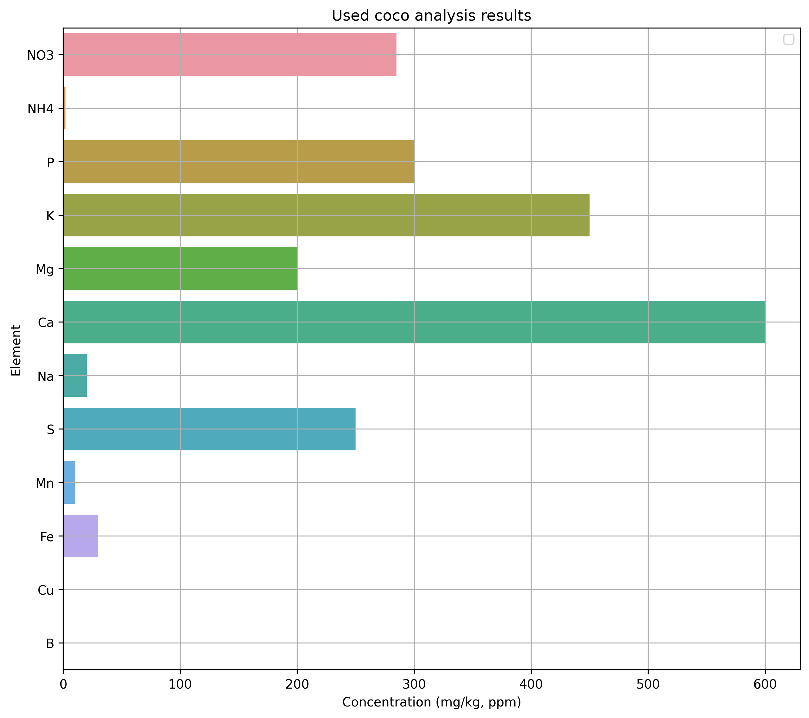
Analysis of used coco from a tomato crop. This analysis uses a DTAP + ammonium acetate process to extract all nutrients from the media. This media had a runoff pH of 6 with an EC of 3.0 mS/cm.
The above image shows you the analysis results of a coco sample that was used to grow a tomato crop. In this analysis, the media is extracted exhaustively using a chelating agent, to ensure that we can get a good idea of all the cations that are present in the media. The chelating agent overcomes the cation exchange capacity of the media, forcing all the cations out – fundamentally exchanging them for sodium or ammonium – and showing you the limits of what could be extracted from the media by the plant.
In this case, the amount of Ca is so high, that it can fundamentally provide most of the Ca required by a plant through its next growing period. Since most of this Ca is going to be present as calcium sulfate and phosphate, it will only be removed quite slowly from the root zone by leachate. The amount of potassium is also quite high, but this potassium is going to go out of the media quite easily and is only likely to last for a short period of time.
In addition to the above mineral content, coco that is reused will often contain a lot of plant material, roots that remained from the previous crop, so the subsequent reuse of the media needs to incorporate adequate enzymatic treatments to help breakdown these organics and ensure that pathogens are not going to be able to use these sources of carbon as an anchor point to attack our plants.
Steps before the crop ends
Because of the above, one of the first steps we need to carry out if we want to reuse media is to ensure that the media is flushed during the last week of crop usage with plain water, such that we can get most of the highly soluble nutrients out of the media so that we don’t need to deal with those nutrients in our calculations. This will remove most of the nitrogen and potassium from the above analysis, giving us media that is easier to use in our next crop.
In addition to this, we will also be preparing our media for the digestion of the root material. Before the last week of cultivation, we will add pondzyme to our plain water flushing at a rate of 0.1g/gal, such that we can get a good amount of enzymes into our media. We should also add some beneficial microbes, like these probiotics, at 0.25g/gal, so that we can get some microbial life into the media that will help us decompose the roots after the plants that are currently in the media will be removed.
How to manage the new crop
Once the crop ends, we will remove the main root ball from the media. There is no need to make an effort to remove all plant material as this would add a lot of labor costs to media reuse. The media should then be allowed to dry, such that the roots that are left behind can then be easily broken up before new plants are placed in the media. Machines to breakup any roots are ideal, although this can also be done manually and easily once all the root material in the media is dead and the roots lose their capacity to hold their structure together.
Once we have dry coco with the root structures broken up, we can then fill up new bags to reuse this media for our next crop. After doing a lot of media analysis and working with several people reusing media, I have found this method works well. If we performed the flushing steps as instructed before, then we can use the media runoff EC as a way to evaluate the type of nutrition needed.
While the runoff EC remains above 1.5mS/cm, we feed a solution containing only potassium nitrate and micronutrients (no phosphorus, sulfates, calcium or magnesium) at 2g/gal of KNO3 + micros. After the runoff EC drops below 1.5mS/cm we return to feeding our normal regime. The idea here is that while the media is above 1.5mS/cm the plant can take all the nutrients it needs from the media, but once the media EC drops below 1.5mS/cm, the media is deprived from these nutrients and we need to provide them again for the plant.
Bear in mind that while the nitrogen content of the above feed seems low (just 73 ppm of N from NO3) there is additional nitrogen that is coming from the decomposition of the organic materials left in the media, which can supplement the nitrogen needs of the plants. Despite the flushing on the last week, there is always some nitrate left from the previous crop. I have found that this is enough to support the plant until the runoff drops below our 1.5mS/cm threshold. After this point, the plant can be grown with its normal nutrition.
Simple is better
Although you would ideally want to find exactly which nutrients are missing or present after each batch of media and adjust your nutrition such that you can get your plants the ideal nutrient composition every time, this is not cost effective or required in practice to obtain healthy plant growth. A media like coco possesses a good degree of nutrient buffering capacity (due to it’s high cation exchange capacity and how much nutrition is accumulated after a crop cycle), so it can provide the plants the nutrition of certain nutrients that they need as long as the nutrients that are most easily leached (K and N) are provided to some degree.
The above strategy is simple and can achieve good results for most large crops that are grown using ample nutrients within their normal nutrient formulations. It is true that this might not work for absolutely all cases (or might need some adjustments depending on media volumes) but I’ve found out it is a great strategy that avoids high analysis costs and the need to create very custom nutrient solutions.
Do you reuse your coco? Let us know which strategy you use and what you think about my strategy!
Are Iron chelates of humic/fulvic acids better or worse than synthetics?
Why Fe nutrition is problematic
Plants need substantial amounts of iron to thrive. However, iron is a finicky element, and will react with many substances to form solids that are unavailable for plant uptake. This is a specially common process under high pH, where iron can form insoluble carbonates, hydroxides, oxides, phosphates and even silicates. For this reason, plant scientists have – for the better part of the last 100 years – looked for ways to make Fe more available to plants, while preventing the need for strategies that aim to lower the pH of the soil, which can be very costly when large amounts of soil need to be amended.
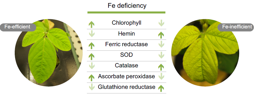
The image above is taken from this paper on Fe deficiencies.
In hydroponics, the situation is not much better. While we can add as much Fe as we want to the hydroponic solution, the above processes still happen and the use of simple Fe salts (such as iron nitrate or iron sulfate) can lead to Fe deficiencies as the iron falls out of solution. This can happen quickly in root zones where plants aggressively increase the pH of solutions through heavy nitrate uptake.
For a better understanding of the basics of soil interactions with microbes, plants and the overall Fe cycle, I suggest reading this review (6).
Synthetic chelates to the rescue
The above problems were alleviated by the introduction of synthetic iron chelates in the mid 20th century. The chelating agents are organic moieties that can wrap around the naked metal ions, binding to their coordination sites. This kills their reactivity and ensures that they do not react with any of the substances that would cause them to become unavailable to plants. Plants can directly uptake the chelates, take the iron and push the chelate back into solution, or they can destroy the chelate and use its carbon within their metabolism.
Chelates can bind Fe very strongly though, and this is not desirable for some plants that do not have the enzymatic machinery required to open these “molecular cages”. Studies with monocots (1) – which are grasses – have often found that these plants respond poorly to Fe supplementation with molecules like Fe(EDDHA), a very powerful chelate. So powerful in fact, that not even the plants can get the Fe out. For these plants, weaker chelates often offer better results, even at higher pH values.
Another problem is that many of the synthetic chelates are not very good at high pH values. When the pH reaches values higher than 7.5, chelates like EDTA and DTPA can have problems competing with the much more strongly insoluble salts that form at these pH values. The chelated forms are always in equilibrium with the non-chelated forms and the minuscule amount of the non-chelated form drops so quickly out of solution that the entire chelate population can be depleted quite quickly. (2)
Chelates that respond well to high pH values, like EDDHA, are often much more expensive. In the case of EDDHA, the presence of a lot of isomers of the EDDHA molecule that are weaker chelates, also creates problems with quality control and with the overall strength of each particular EDDHA source. The EDDHA is only as good as its purification process, which makes good sources even more expensive (3, 4).
An additional concern is the oxidation state of the Fe. While Fe chelates are usually prepared using ferrous iron (Fe2+), these iron chelates are quickly oxidized in solution to their ferric iron (Fe3+) counterparts, especially when the solution is aerated to maintain high levels of oxygen. Since Fe3+ is both more tightly bound to chelates and more reactive when free – so more toxic when taken up without reduction – plants can have an even harder time mining Fe3+ out of chelates (5, 7).
Then there are naturally occurring chelates
There are many organic molecules that can form bonds with the coordination sites of Fe ions. Some of the reviews cited before go into some depth on the different groups of organic molecules that are excreted by both plants and microorganisms as a repose to Fe deficiency that can lead to improved Fe transport into plants. Some of these compounds are also reductive in nature, such that they can not only transport the Fe, but reduce it to its ferrous form such that it can be handled more easily by plants.
Among the organic compounds that can be used for Fe chelation, humic and fulvic acids have attracted attention, as they can be obtained at significantly low costs and are approved for organic usage under several regulations. You can read more about these substances in some of my previous posts about them (8, 9). In particular, humic acids are more abundant and are formed by larger and more complex molecules compared to fulvic acids.
The ability of these substances to chelate Fe is much weaker than that of synthetic chelates. The pKb shows us the strength of the binding equilibrium of the chelate with the free metal ion (you can see the values for many metals and chelating agents here). The value for EDTA is 21.5 while that of most humic and fulvic acids is in the 4-6 range (10). This is a logarithmic scale, so the difference in binding strength is enormous. To put things into perspective, this difference in binding strength is of the same magnitude as the difference between the mass of a grain of sand and a cruise ship.
Comparing synthetic and fulvic/humic acid chelates
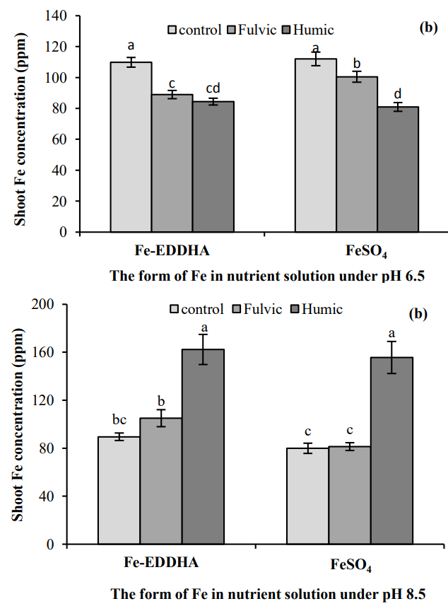
There aren’t many studies comparing synthetic and humic/fulvic acid chelates. One of the most explicit ones (11) compares solutions of Fe sulfate (which we can consider unchelated) and Fe(EDDHA) after additions of fulvic or humic acids in the growth of Pistachio plants. At pH values close to those generally used in hydroponics (6.5) there is hardly any difference between any of the treatments while at higher pH values we have substantially better uptake of Fe in both the EDDHA and unchelated iron treatments when supplemented with either fulvic acid or humic acid.
Images at pH 8.5 of Fe in shoots from the Pistachio study (11)
The idea of using humic acids as a compliment of traditional chelate based fertilization to alleviate high fertilization costs has also been studied in citrus (13). This study confirms some of the findings of the previous one, where additions of humic acids to solutions already containing Fe(EDDHA) provided a more beneficial role than simply the use of the pure humic acid substances or pure Fe(EDDHA) fertilization. Another study on citrus (14) showed that humic acid applications could in fact provide Fe supplementation in calcareous soils (these are soils with high pH values). This shows how humic acid fertilization can rival Fe-EDDHA fertilization.
In another study of leonardite iron humate sources and EDDHA in soybean roots (12) it is apparent that accumulation of Fe in shoots and roots is much worse under the humic acid treatments. In the conclusions of the paper, it is highlighted that the high molecular mass of the leonardite constituents might block the roots of the soybean plants, therefore making it difficult for the plant to transport Fe. However, this study does show that the accumulation of these humic acids in the root zone does promote a decrease in the expression of genes that create Fe transporters and Fe reducing enzymes, pointing that the plant is indeed under less Fe deficiency stress. Another important point is that cycling the humic acid application promotes the absorption of accumulated humic acids, cleaning the roots and allowing for better transport of the Fe in the roots.
In a separate study with humic acid + FeSO4 applications compared to Fe(EDDHA) in sweet cherry (13) it was found that the humic acid, when supplemented with unchelated iron, increased Fe tissue as much as the Fe(EDDHA) applications. This was consistent across two separate years, with the second year showing a statistically significant increase of the humic acid treatment over the Fe(EDDHA).
How does this work
An interesting point – as I mentioned before – is that humic/fulvic acids are incredibly weak chelating agents. This means that they should release their Fe to the bulk of the solution, which should lead to Fe depletion and deficiencies, as the Fe precipitating mechanisms are thermodynamically much more stable. However this is not what we consistently observe in the studies of Fe nutrition that try to use humic/fulvic acids, either with or without the presence of additional synthetic chelates.
The reason seems to be related with the kinetics of Fe release from these substances. While the stability constants of the chelates are weak – therefore they will release and precipitate in the long term – the bulkiness of the ligands and the complex structures surrounding the metals, makes it hard for the metal to actually escape from the chelate structures around it. However, the fact that the bonding is thermodynamically weak, ensures that the metal can be easily transported once it leaves the organic chelate structure.
Another point is that humic/fulvic substances are reductive in nature, which means that they will protect Fe2+ from oxidation by either microbes or oxygen dissolved in solution. They are also sometimes able to reduce Fe3+ present in solution back to Fe2+, which can help with the uptake of this Fe by the plant’s root system.
The nature of the above structures and their reductive power depends fundamentally on the actual humic/fulvic acid used, so – as with all cases pertaining to fulvic/humic substances – the source you use will play a big role in determining the final outcome you get.
What chelates are the best?
Current research shows that Fe(EDDHA) and similar chelates, despite their high stability constants, are not perfect. While they can provide ample iron for dicots and can cure Fe deficiencies in the large majority of cases for these plants, these strong chelates are often very expensive and their use as sole Fe sources might be impractical for many cases in traditional agriculture and hydroponics/soilless growing.
The use of humic/fulvic acids complimented with either unchelated Fe or with some lower proportion of stronger iron chelates, seems to be a better overall choice in terms of both plant uptake and economic expense. As shown by several studies mentioned in this post, the effect of humic/fulvic acids and synthetic chelates might actually be synergistic, with both providing different advantages that can be complimentary in hydroponic solutions. These humic/fulvic acid solutions might also be much more favorable for monocot species, where the use of highly stable Fe(EDDHA) chelating agents does not cure deficiency symptoms.
The take away here is that chemical chelate strength is not the only thing to consider. The kinetics of the chelate dissociations, as well as how the chelates interact with the root system, for example how the plant can actually take the Fe outside of the chelating system, are all very important to establish whether the Fe is effectively absorbed and transported by the plants.
Please note that the topic of Fe nutrition is extremely extensive and while the above is intended to be a short introduction to the topic of humic/fulvic acids and how they compare to synthetic chelates, it is by no means an exhaustive literature review.
Are you using fulvic or humic acids for Fe nutrition? Let us know what your experience is in the comments below.