Peptide Biostimulants in Plants: What They Are and What They Actually Do
Peptide biostimulants have gained significant attention in horticulture and hydroponics, with claims ranging from modest growth improvements to dramatic yield boosts. In this post, I want to examine what the peer-reviewed science actually tells us about these products. The evidence shows that peptide-based biostimulants can deliver measurable benefits under specific conditions, but their mechanisms remain incompletely understood and results vary considerably depending on source material, application method, and growing environment.
What exactly are peptide biostimulants?
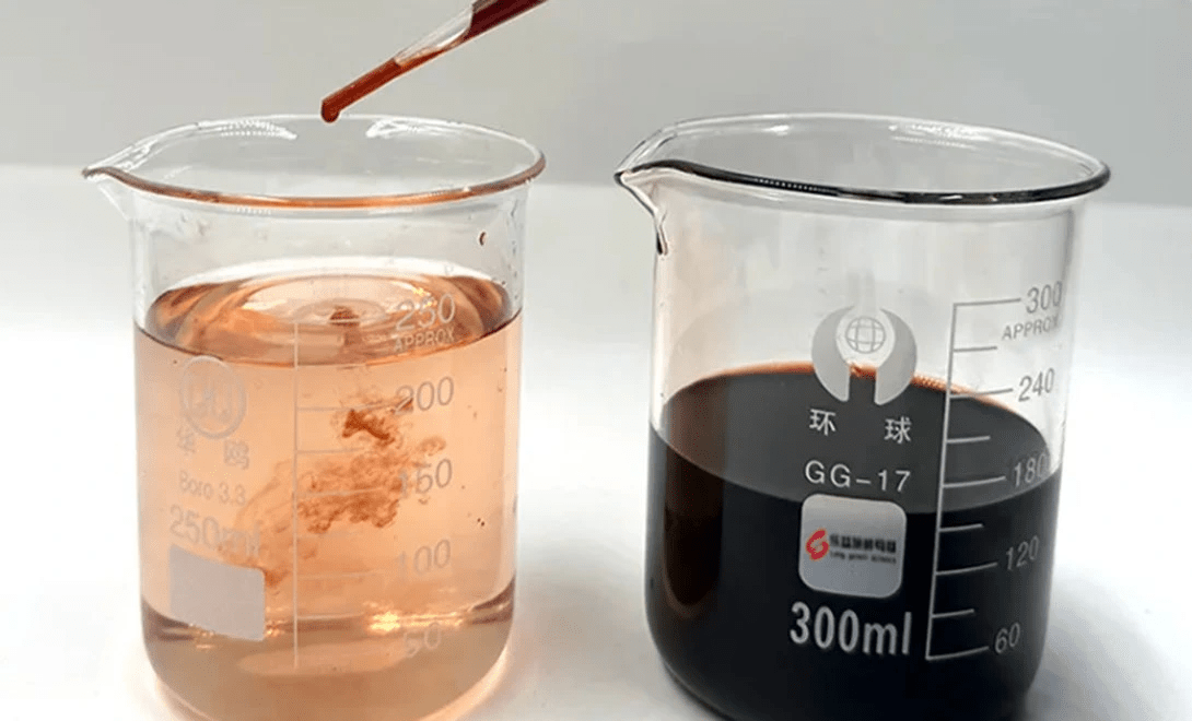
Peptide biostimulants are products containing short chains of amino acids, typically 2 to 100 amino acids in length. Most commercial products fall under the broader category of protein hydrolysates, which are mixtures of free amino acids, oligopeptides, and polypeptides resulting from partial protein breakdown (1). These products come from animal-derived materials (leather by-products, blood meal, fish waste, chicken feathers, casein) or plant-derived materials (legume seeds, alfalfa, vegetable by-products) (2).
The production method matters significantly. Chemical hydrolysis using acids or alkalis tends to produce more free amino acids and smaller peptides, while enzymatic hydrolysis preserves more intact peptides and a broader range of molecular sizes (1). Plant-derived protein hydrolysates produced through enzymatic processes generally show higher biostimulant activity in research settings compared to chemically hydrolyzed animal-derived products (3).
Why this pattern exists remains incompletely explained. Is the advantage due to specific peptide sequences unique to plant proteins? The lower free amino acid content reducing phytotoxicity risk? Larger average peptide size? Lower salt content from avoiding harsh chemical hydrolysis? The research establishes the trend but does not conclusively identify the causal mechanism. This matters because without understanding why plant-derived products work better, predicting which specific formulations will perform well becomes more guesswork than science.
| Source Type | Common Raw Materials | Hydrolysis Method | Typical Composition |
|---|---|---|---|
| Plant-derived | Legume seeds, soybean, alfalfa | Enzymatic | Higher peptide content, broader amino acid profile |
| Animal-derived | Fish meal, feathers, blood meal | Chemical | Higher free amino acid content, narrower profile |
How do they work in plants?
The honest answer is that researchers are still piecing together the full picture. As one comprehensive review puts it, knowledge on their mode of action is still piecemeal (1). That said, several mechanisms have been demonstrated in controlled experiments.
Hormone-like activity is among the most frequently cited mechanisms. Studies using corn coleoptile elongation tests and gibberellin-deficient dwarf pea plants have shown that certain protein hydrolysates exhibit both auxin-like and gibberellin-like activity (3). In one study, application of a plant-derived protein hydrolysate increased shoot length in dwarf pea plants by 33% compared to untreated controls.
However, these bioassays deserve scrutiny. Coleoptile elongation tests and dwarf mutant responses are extremely sensitive screening tools designed to detect minute hormonal activity. They tell us that something hormone-like is present, but they do not predict whether those effects translate to meaningful outcomes in production systems with normal hormone homeostasis. A compound can show auxin-like behavior in a coleoptile assay yet have negligible impact on a mature plant with intact hormone synthesis and transport. The research demonstrates hormone-like activity, but the operational significance for commercial growing remains largely assumed rather than proven.
The auxin-like activity appears connected to both the tryptophan content in these products (a precursor to the plant hormone IAA) and specific bioactive peptides like the 12-amino-acid root hair promoting peptide isolated from soybean-derived hydrolysates (2).
Enhanced nitrogen metabolism represents another documented pathway. Gene expression studies show that protein hydrolysate application upregulates key nitrogen transporters (NRT2.1, NRT2.3) and amino acid transporters in roots and leaves (4). The enzymes involved in nitrogen assimilation, including nitrate reductase and glutamine synthetase, also show increased activity following treatment (1). Additionally, peptide biostimulants can improve micronutrient availability through chelation effects (2).
What does the experimental evidence actually show?
When examining controlled experiments, the reported improvements require careful interpretation. The frequently cited studies show percentage gains that look impressive on paper but come with important caveats about baseline conditions.
In greenhouse tomato trials, legume-derived protein hydrolysates increased shoot dry weight by 21%, root dry weight by 35%, and root surface area by 26% in tomato cuttings (3). However, these cuttings were grown in substrate culture with suboptimal nutrient availability. The 35% root dry weight increase translated to an absolute gain of roughly 0.3 grams per plant over 12 days on plants with small initial biomass. Whether this scales to mature plants in optimized systems remains unclear.
Studies reporting 50% yield increases in baby lettuce (2) used reduced nutrient conditions (50% of standard nitrogen). This is a common pattern: the largest percentage improvements appear when baseline nutrition is deliberately limited. The tomato fruit quality improvements showed smaller changes, typically 10-15%, in field-grown plants (2).
For stress tolerance, protein hydrolysates have shown measurable effects through activation of antioxidant systems, osmotic adjustment, and modulation of stress-related hormones (1). Research on drought stress recovery in tomato found that certain plant-derived protein hydrolysates were 62-75% more effective at enhancing recovery compared to untreated controls (5), though again these were substrate-grown plants under deliberately induced stress conditions.
The hydroponic data gap
Here is an uncomfortable truth: nearly all the research cited above comes from soil-based or substrate culture systems, not true hydroponics. The tomato studies used peat-based growing media. The lettuce trials were conducted in soil with modified nutrient solutions.
I found no peer-reviewed studies testing peptide biostimulants in nutrient film technique, deep water culture, or aeroponics under controlled conditions. The extrapolation from substrate culture to recirculating hydroponic systems rests on assumptions about peptide stability in solution, interactions with synthetic nutrient salts, and whether root uptake mechanisms differ without substrate.
Hydroponic systems have fundamentally different dynamics around root exudates, microbial populations, oxygen availability, and nutrient contact time. As a hydroponic grower, you are essentially conducting your own experiment when using these products, because the research has not caught up to your growing method yet.
The caveats you need to know
Here is where I need to pump the brakes on any excessive enthusiasm. Not all studies show positive effects, and some show no significant benefit at all.
Several studies on animal-derived products found minimal or non-significant effects on crops including endive, spinach, carrot, and okra under field conditions (2). The variability depends heavily on protein source, production process, crop species, application timing, concentration, and environmental conditions.
There is also the phenomenon called general amino acid inhibition. Excessive uptake of free amino acids through foliar application can cause phytotoxicity, intracellular amino acid imbalance, and growth suppression (2). This occurs more commonly with animal-derived products that contain higher proportions of free amino acids.
Most research has been conducted with specific commercial formulations under controlled conditions. The impressive percentage improvements often come from comparing treated plants to completely untreated controls, not to plants receiving optimized nutrition programs.
Practical recommendations for hydroponic growers
If you want to experiment with peptide biostimulants, plant-derived products from legume sources using enzymatic hydrolysis show more consistent results in available research (3), though remember this research was not conducted in true hydroponic systems. Start with manufacturer-recommended concentrations, as more is not better. Research suggests foliar applications at 2.5-5 ml/L have shown benefits without phytotoxicity (4).
Be realistic about what you are testing. If your system is already optimized, you are operating in the regime where these products show the smallest benefits. Research shows more pronounced effects under nutrient limitations, drought stress, or other challenges (6). A 30% improvement in a stressed plant may still leave it performing worse than an unstressed control.
Do not expect peptide biostimulants to replace proper nutrition or mask fundamental problems. They work alongside, not instead of, a well-designed nutrient program (5).
Most importantly, treat any trial as an actual experiment. Run side-by-side comparisons with untreated controls. Measure actual outcomes, not subjective impressions. The absence of hydroponic-specific research means you cannot simply apply published percentage improvements to your situation.
The bottom line
Peptide biostimulants represent a legitimate category of agricultural inputs with demonstrated effects on plant physiology in controlled research settings. The science supports claims of hormone-like activity in sensitive bioassays, enhanced nitrogen metabolism at the gene expression level, improved root development in substrate culture, and stress tolerance mechanisms under laboratory conditions.
The evidence base has three major limitations. First, the most impressive percentage gains come from experiments using suboptimal baseline conditions. Second, nearly all research has been conducted in soil or substrate systems rather than true hydroponics. Third, the mechanisms explaining why certain formulations outperform others remain poorly understood.
For hydroponic growers, these products deserve consideration as experimental tools, not proven solutions. The physiology is real, but the operational benefits in optimized recirculating systems are unknown. If you trial peptide biostimulants, design proper experiments with controls and measured outcomes. Treat manufacturer claims with skepticism. Recognize that you are working ahead of the research, not following it.
Have you tried peptide biostimulants in your hydroponic system? What results did you observe? Let us know in the comments below!